Partition based time series clustering in sktime#

Partition based clustering algorithms for time series are those where k clusters are created from n time series. Each time series inside a cluster are homogeneous (similar) to each other and heterogeneous (dissimilar) to those outside the cluster.

To measure homogeneity and place a time series into a cluster, a metrics is used (normally a distance). This metric is used to compare a time series to k other time series that are representations of each cluster. These representations are derived using a statistical sampling technique from when the model was trained. The time series is then assigned to the cluster that is most similar (or has the best score based on the metric), and is said to be a part of that cluster.

Currently, in Sktime there are 2 supported partition algorithms supported. They are: K-means and K-medoids. These will be demonstrated below

Imports#

[1]:

from sklearn.model_selection import train_test_split

from sktime.clustering.k_means import TimeSeriesKMeans
from sktime.clustering.k_medoids import TimeSeriesKMedoids
from sktime.clustering.utils.plotting._plot_partitions import plot_cluster_algorithm
from sktime.datasets import load_arrow_head

Load data#

[2]:

X, y = load_arrow_head(return_X_y=True)
X_train, X_test, y_train, y_test = train_test_split(X, y)
print(X_train.shape, y_train.shape, X_test.shape, y_test.shape)

(158, 1) (158,) (53, 1) (53,)

K-partition algorithms#

K-partition algorithms are those that seek to create k clusters and assign each time series to a cluster using a distance measure. In Sktime the following are currently supported:

K-means - one of the most well known clustering algorithms. The goal of the K-means algorithm is to minimise a criterion known as the inertia or within-cluster sum-of-squares (uses the mean of the values in a cluster as the center).

K-medoids - A similar algorithm to K-means but instead of using the mean of each cluster to determine the center, the median series is used. Algorithmically the common way to approach these k-partition algorithms is known as Lloyds algorithm. This is an iterative process that involves:

Initialisation

Assignment

Updating centroid

Repeat assignment and updating until convergence

Center initialisation#

Center initialisation is the first step and has been found to be critical in obtaining good results. There are three main center initialisation that will now be outlined:

K-means, K-medoids supported center initialisation:
- Random - This is where each sample in the training dataset is randomly assigned to a cluster and update centers is run based on these random assignments i.e. for k-means the mean of these randomly assigned clusters is used and for k-medoids the median of these randomly assigned clusters is used as the initial center.
- Forgy - This is where k random samples are chosen from the training dataset
- K-means++ - This is where the first center is randomly chosen from the training dataset. Then for all the other time series in the training dataset, the distance between them and the randomly selected center is taken. The next center is then chosen from the training dataset so that the probability of being chosen is proportional to the distance (i.e. the greater the distance the more likely the time series will be chosen). The remaining centers are then generated using the same method. This means each center will be generated so that the probability of a being chosen becomes proportional to its closest center (i.e. the further from an already chosen center the more likely it will be chosen).
```
</li>
```

These three cluster initialisation algorithms have been implemented and can be chosen to use when constructing either k-means or k-medoids partitioning algorithms by parsing the string values ‘random’ for random initialisation, ‘forgy’ for forgy and ‘k-means++’ for k-means++.

Assignment (distance measure)#

How a time series is assigned to a cluster is based on its distance from it to the cluster center. This means for some k-partition approaches, different distances can be used to get different results. While details on each of the distances won’t be discussed here the following are supported, and their parameter values are defined:

K-means, K-medoids supported distances:
- Euclidean - parameter string ‘euclidean’
- DTW - parameter string ‘dtw’
- DDTW - parameter string ‘ddtw’
- WDTW - parameter string ‘wdtw’
- WDDTW - parameter string ‘wddtw’
- LCSS - parameter string ‘lcss’
- ERP - parameter string ‘erp’
- EDR - parameter string ‘edr’
- MSM - parameter string ‘msm’
```
</li>
```

Updating centroids#

Center updating is key to the refinement of clusters to improve their quality. How this is done depends on the algorithm, but the following are supported

K-means
- Mean average - This is a standard mean average creating a new series that is that average of all the series inside the cluster. Ideal when using euclidean distance. Can be specified to use by parsing ‘means’ as the parameter for averaging_algorithm to k-means
- DTW Barycenter averaging (DBA) - This is a specialised averaging metric that is intended to be used with the dtw distance measure as it used the dtw matrix path to account for alignment when determining an average series. This provides a much better representation of the mean for time series. Can be specified to use by parsing ‘dba’ as the parameter for averaging_algorithm to k-means.
```
</li>
<li> K-medoids
    <ul>
        <li>Median - Standard meadian which is the series in the middle of
        all series in a cluster. Used by default by k-medoids</li>
    </ul>
```

K-means#

[3]:

k_means = TimeSeriesKMeans(
    n_clusters=5,  # Number of desired centers
    init_algorithm="forgy",  # Center initialisation technique
    max_iter=10,  # Maximum number of iterations for refinement on training set
    metric="euclidean",  # Distance metric to use. Choose "dtw" for dynamic time warping
    averaging_method="mean",  # Averaging technique to use
    random_state=1,
)

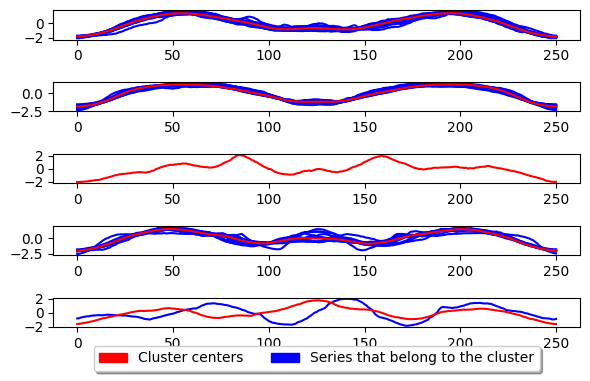
k_means.fit(X_train)
plot_cluster_algorithm(k_means, X_test, k_means.n_clusters)

<Figure size 360x720 with 0 Axes>

../../_images/examples_clustering_partition_based_clustering_5_1.png

K-medoids#

[4]:

k_medoids = TimeSeriesKMedoids(
    n_clusters=5,  # Number of desired centers
    init_algorithm="forgy",  # Center initialisation technique
    max_iter=10,  # Maximum number of iterations for refinement on training set
    verbose=False,  # Verbose
    metric="euclidean",  # Distance metric. Use "dtw" for dynamic time warping
    random_state=1,
)

k_medoids.fit(X_train)
plot_cluster_algorithm(k_medoids, X_test, k_medoids.n_clusters)

<Figure size 500x1000 with 0 Axes>

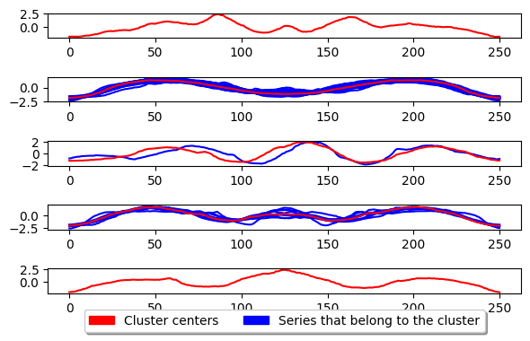
../../_images/examples_clustering_partition_based_clustering_7_1.png

The above shows the basic usage for K-medoids. This algorithm works essentially the same as K-means but instead of updating the center by taking the mean of the series inside the cluster, it takes the median series. This means the center is an existing series in the dataset and NOT a generated one. The parameter key to k-medoids is the metric and is what we can adjust to improve performance for time series. An example of using dtw as the metric is given below.

[5]:

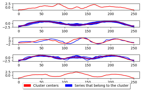
k_medoids = TimeSeriesKMedoids(
    n_clusters=5,  # Number of desired centers
    init_algorithm="forgy",  # Center initialisation technique
    max_iter=10,  # Maximum number of iterations for refinement on training set
    metric="euclidean",  # Distance metric. Use "dtw" for dynamic time warping
    random_state=1,
)

k_medoids.fit(X_train)
plot_cluster_algorithm(k_medoids, X_test, k_medoids.n_clusters)

<Figure size 500x1000 with 0 Axes>

../../_images/examples_clustering_partition_based_clustering_9_1.png

Generated using nbsphinx. The Jupyter notebook can be found here.