

Probabilistic Forecasting with sktime

Probabilistic Forecasting with sktime
originally presented at pydata Berlin 2022, see there for video presentation
Overview of this notebook
quick start - probabilistic forecasting
disambiguation - types of probabilistic forecasts
details: probabilistic forecasting interfaces
metrics for, and evaluation of probabilistic forecasts
advanced composition: pipelines, tuning, reduction
extender guide
contributor credits
[1]:
import warnings

warnings.filterwarnings("ignore")
Quick Start - Probabilistic Forecasting with sktime
… works exactly like the basic forecasting workflow, replace predict by a probabilistic method!
[2]:
from sktime.datasets import load_airline
from sktime.forecasting.arima import ARIMA

# step 1: data specification
y = load_airline()
# step 2: specifying forecasting horizon
fh = [1, 2, 3]
# step 3: specifying the forecasting algorithm
forecaster = ARIMA()
# step 4: fitting the forecaster
forecaster.fit(y, fh=[1, 2, 3])
# step 5: querying predictions
y_pred = forecaster.predict()

# for probabilistic forecasting:
#   call a probabilistic forecasting method after or instead of step 5
y_pred_int = forecaster.predict_interval(coverage=0.9)
y_pred_int
[2]:
| Number of airline passengers | ||
|---|---|---|
| 0.9 | ||
| lower | upper | |
| 1961-01 | 371.535093 | 481.554608 |
| 1961-02 | 344.853205 | 497.712761 |
| 1961-03 | 324.223995 | 508.191104 |
probabilistic forecasting methods in ``sktime``:
forecast intervals -
predict_interval(fh=None, X=None, coverage=0.90)forecast quantiles -
predict_quantiles(fh=None, X=None, alpha=[0.05, 0.95])forecast variance -
predict_var(fh=None, X=None, cov=False)distribution forecast -
predict_proba(fh=None, X=None, marginal=True)
To check which forecasters in sktime support probabilistic forecasting, use the registry.all_estimators utility and search for estimators which have the capability:pred_int tag (value True).
For composites such as pipelines, a positive tag means that logic is implemented if (some or all) components support it.
[3]:
from sktime.registry import all_estimators

all_estimators(
    "forecaster", filter_tags={"capability:pred_int": True}, as_dataframe=True
)
[3]:
| name | object | |
|---|---|---|
| 0 | ARCH | <class 'sktime.forecasting.arch._uarch.ARCH'> |
| 1 | ARIMA | <class 'sktime.forecasting.arima.ARIMA'> |
| 2 | AutoARIMA | <class 'sktime.forecasting.arima.AutoARIMA'> |
| 3 | AutoETS | <class 'sktime.forecasting.ets.AutoETS'> |
| 4 | BATS | <class 'sktime.forecasting.bats.BATS'> |
| 5 | BaggingForecaster | <class 'sktime.forecasting.compose._bagging.Ba... |
| 6 | ColumnEnsembleForecaster | <class 'sktime.forecasting.compose._column_ens... |
| 7 | ConformalIntervals | <class 'sktime.forecasting.conformal.Conformal... |
| 8 | DynamicFactor | <class 'sktime.forecasting.dynamic_factor.Dyna... |
| 9 | FhPlexForecaster | <class 'sktime.forecasting.compose._fhplex.FhP... |
| 10 | ForecastX | <class 'sktime.forecasting.compose._pipeline.F... |
| 11 | ForecastingGridSearchCV | <class 'sktime.forecasting.model_selection._tu... |
| 12 | ForecastingPipeline | <class 'sktime.forecasting.compose._pipeline.F... |
| 13 | ForecastingRandomizedSearchCV | <class 'sktime.forecasting.model_selection._tu... |
| 14 | ForecastingSkoptSearchCV | <class 'sktime.forecasting.model_selection._tu... |
| 15 | NaiveForecaster | <class 'sktime.forecasting.naive.NaiveForecast... |
| 16 | NaiveVariance | <class 'sktime.forecasting.naive.NaiveVariance'> |
| 17 | Permute | <class 'sktime.forecasting.compose._pipeline.P... |
| 18 | Prophet | <class 'sktime.forecasting.fbprophet.Prophet'> |
| 19 | SARIMAX | <class 'sktime.forecasting.sarimax.SARIMAX'> |
| 20 | SquaringResiduals | <class 'sktime.forecasting.squaring_residuals.... |
| 21 | StatsForecastARCH | <class 'sktime.forecasting.arch._statsforecast... |
| 22 | StatsForecastAutoARIMA | <class 'sktime.forecasting.statsforecast.Stats... |
| 23 | StatsForecastAutoCES | <class 'sktime.forecasting.statsforecast.Stats... |
| 24 | StatsForecastAutoETS | <class 'sktime.forecasting.statsforecast.Stats... |
| 25 | StatsForecastAutoTheta | <class 'sktime.forecasting.statsforecast.Stats... |
| 26 | StatsForecastGARCH | <class 'sktime.forecasting.arch._statsforecast... |
| 27 | StatsForecastMSTL | <class 'sktime.forecasting.statsforecast.Stats... |
| 28 | TBATS | <class 'sktime.forecasting.tbats.TBATS'> |
| 29 | ThetaForecaster | <class 'sktime.forecasting.theta.ThetaForecast... |
| 30 | TransformedTargetForecaster | <class 'sktime.forecasting.compose._pipeline.T... |
| 31 | UnobservedComponents | <class 'sktime.forecasting.structural.Unobserv... |
| 32 | VAR | <class 'sktime.forecasting.var.VAR'> |
| 33 | VECM | <class 'sktime.forecasting.vecm.VECM'> |
| 34 | YfromX | <class 'sktime.forecasting.compose._reduce.Yfr... |
What is probabilistic forecasting?
Intuition
produce low/high scenarios of forecasts
quantify uncertainty around forecasts
produce expected range of variation of forecasts
Interface view
Want to produce “distribution” or “range” of forecast values,
at time stamps defined by forecasting horizon fh
given past data y (series), and possibly exogeneous data X
Input, to fit or predict: fh, y, X
Output, from predict_probabilistic: some “distribution” or “range” object
Big caveat: there are multiple possible ways to model “distribution” or “range”!
Used in practice and easily confused! (and often, practically, confused!)
Formal view (endogeneous, one forecast time stamp)
Let \(y(t_1), \dots, y(t_n)\) be observations at fixed time stamps \(t_1, \dots, t_n\).
(we consider \(y\) as an \(\mathbb{R}^n\)-valued random variable)
Let \(y'\) be a (true) value, which will be observed at a future time stamp \(\tau\).
(we consider \(y'\) as an \(\mathbb{R}\)-valued random variable)
We have the following “types of forecasts” of \(y'\):
Name |
param |
prediction/estimate of |
|
|---|---|---|---|
point forecast |
conditional expectation \(\mathbb{E}[y'\|y]\) |
|
|
variance forecast |
conditional variance \(Var[y'\|y]\) |
|
|
quantile forecast |
\(\alpha\in (0,1)\) |
\(\alpha\)-quantile of \(y'\|y\) |
|
interval forecast |
\(c\in (0,1)\) |
\([a,b]\) s.t. \(P(a\le y' \le b\| y) = c\) |
|
distribution forecast |
the law/distribution of \(y'\|y\) |
|
Notes:
different forecasters have different capabilities!
metrics, evaluation & tuning are different by “type of forecast”
compositors can “add” type of forecast! Example: bootstrap
More formal details & intuition:
a “point forecast” is a prediction/estimate of the conditional expectation \(\mathbb{E}[y'|y]\). Intuition: “out of many repetitions/worlds, this value is the arithmetic average of all observations”.
a “variance forecast” is a prediction/estimate of the conditional expectation \(Var[y'|y]\). Intuition: “out of many repetitions/worlds, this value is the average squared distance of the observation to the perfect point forecast”.
a “quantile forecast”, at quantile point \(\alpha\in (0,1)\) is a prediction/estimate of the \(\alpha\)-quantile of \(y'|y\), i.e., of \(F^{-1}_{y'|y}(\alpha)\), where \(F^{-1}\) is the (generalized) inverse cdf = quantile function of the random variable y’|y. Intuition: “out of many repetitions/worlds, a fraction of exactly \(\alpha\) will have equal or smaller than this value.”
an “interval forecast” or “predictive interval” with (symmetric) coverage \(c\in (0,1)\) is a prediction/estimate pair of lower bound \(a\) and upper bound \(b\) such that \(P(a\le y' \le b| y) = c\) and \(P(y' \gneq b| y) = P(y' \lneq a| y) = (1 - c) /2\). Intuition: “out of many repetitions/worlds, a fraction of exactly \(c\) will be contained in the interval \([a,b]\), and being above is equally likely as being below”.
a “distribution forecast” or “full probabilistic forecast” is a prediction/estimate of the distribution of \(y'|y\), e.g., “it’s a normal distribution with mean 42 and variance 1”. Intuition: exhaustive description of the generating mechanism of many repetitions/worlds.
Notes:
lower/upper of interval forecasts are quantile forecasts at quantile points \(0.5 - c/2\) and \(0.5 + c/2\) (as long as forecast distributions are absolutely continuous).
all other forecasts can be obtained from a full probabilistic forecasts; a full probabilistic forecast can be obtained from all quantile forecasts or all interval forecasts.
there is no exact relation between the other types of forecasts (point or variance vs quantile)
in particular, point forecast does not need to be median forecast aka 0.5-quantile forecast. Can be \(\alpha\)-quantile for any \(\alpha\)!
Frequent confusion in literature & python packages:
coverage
cvs quantile\alphacoverage
cvs significancep = 1-cquantile of lower interval bound,
p/2, vspinterval forecasts vs related, but substantially different concepts: confidence interval on predictive mean; Bayesian posterior or credibility interval of the predictive mean
all forecasts above can be Bayesian, confusion: “posteriors are different” or “have to be evaluated differently”
Probabilistic forecasting interfaces in sktime
This section:
walkthrough of probabilistic predict methods
use in update/predict workflow
multivariate and hierarchical data
All forecasters with tag capability:pred_int provide the following:
forecast intervals -
predict_interval(fh=None, X=None, coverage=0.90)forecast quantiles -
predict_quantiles(fh=None, X=None, alpha=[0.05, 0.95])forecast variance -
predict_var(fh=None, X=None, cov=False)distribution forecast -
predict_proba(fh=None, X=None, marginal=True)
Generalities:
methods do not change state, multiple can be called
fhis optional, if passed lateexogeneous data
Xcan be passed
[4]:
import numpy as np

from sktime.datasets import load_airline
from sktime.forecasting.theta import ThetaForecaster

# until fit, identical with the simple workflow
y = load_airline()

fh = np.arange(1, 13)

forecaster = ThetaForecaster(sp=12)
forecaster.fit(y, fh=fh)
[4]:
ThetaForecaster(sp=12)Please rerun this cell to show the HTML repr or trust the notebook.
ThetaForecaster(sp=12)
fh - forecasting horizon (not necessary if seen in fit)coverage, float or list of floats, default=0.9pandas.DataFramefhcoverageEntries = forecasts of lower/upper interval at nominal coverage in 2nd lvl, for var in 1st lvl, for time in row
[5]:
coverage = 0.9
y_pred_ints = forecaster.predict_interval(coverage=coverage)
y_pred_ints
[5]:
| Number of airline passengers | ||
|---|---|---|
| 0.9 | ||
| lower | upper | |
| 1961-01 | 418.280121 | 464.281951 |
| 1961-02 | 402.215881 | 456.888055 |
| 1961-03 | 459.966113 | 522.110500 |
| 1961-04 | 442.589309 | 511.399214 |
| 1961-05 | 443.525027 | 518.409480 |
| 1961-06 | 506.585814 | 587.087737 |
| 1961-07 | 561.496768 | 647.248956 |
| 1961-08 | 557.363322 | 648.062363 |
| 1961-09 | 477.658055 | 573.047752 |
| 1961-10 | 407.915090 | 507.775355 |
| 1961-11 | 346.942924 | 451.082017 |
| 1961-12 | 394.708221 | 502.957142 |
pretty-plotting the predictive interval forecasts:
[6]:
from sktime.utils import plotting

# also requires predictions
y_pred = forecaster.predict()

fig, ax = plotting.plot_series(
    y, y_pred, labels=["y", "y_pred"], pred_interval=y_pred_ints
)

ax.legend();

multiple coverages:
[7]:
coverage = [0.5, 0.9, 0.95]
y_pred_ints = forecaster.predict_interval(coverage=coverage)
y_pred_ints
[7]:
| Number of airline passengers | ||||||
|---|---|---|---|---|---|---|
| 0.50 | 0.90 | 0.95 | ||||
| lower | upper | lower | upper | lower | upper | |
| 1961-01 | 431.849266 | 450.712806 | 418.280121 | 464.281951 | 413.873755 | 468.688317 |
| 1961-02 | 418.342514 | 440.761421 | 402.215881 | 456.888055 | 396.979011 | 462.124925 |
| 1961-03 | 478.296822 | 503.779790 | 459.966113 | 522.110500 | 454.013504 | 528.063109 |
| 1961-04 | 462.886144 | 491.102379 | 442.589309 | 511.399214 | 435.998232 | 517.990291 |
| 1961-05 | 465.613670 | 496.320837 | 443.525027 | 518.409480 | 436.352089 | 525.582418 |
| 1961-06 | 530.331440 | 563.342111 | 506.585814 | 587.087737 | 498.874797 | 594.798754 |
| 1961-07 | 586.791063 | 621.954661 | 561.496768 | 647.248956 | 553.282845 | 655.462879 |
| 1961-08 | 584.116789 | 621.308897 | 557.363322 | 648.062363 | 548.675556 | 656.750129 |
| 1961-09 | 505.795123 | 544.910684 | 477.658055 | 573.047752 | 468.520987 | 582.184821 |
| 1961-10 | 437.370840 | 478.319605 | 407.915090 | 507.775355 | 398.349800 | 517.340645 |
| 1961-11 | 377.660798 | 420.364142 | 346.942924 | 451.082017 | 336.967779 | 461.057162 |
| 1961-12 | 426.638370 | 471.026993 | 394.708221 | 502.957142 | 384.339408 | 513.325954 |
fh - forecasting horizon (not necessary if seen in fit)alpha, float or list of floats, default = [0.1, 0.9]pandas.DataFramefhalphaEntries = forecasts of quantiles at quantile point in 2nd lvl, for var in 1st lvl, for time in row
[8]:
alpha = [0.1, 0.25, 0.5, 0.75, 0.9]
y_pred_quantiles = forecaster.predict_quantiles(alpha=alpha)
y_pred_quantiles
[8]:
| Number of airline passengers | |||||
|---|---|---|---|---|---|
| 0.10 | 0.25 | 0.50 | 0.75 | 0.90 | |
| 1961-01 | 423.360378 | 431.849266 | 441.281036 | 450.712806 | 459.201694 |
| 1961-02 | 408.253656 | 418.342514 | 429.551968 | 440.761421 | 450.850279 |
| 1961-03 | 466.829089 | 478.296822 | 491.038306 | 503.779790 | 515.247523 |
| 1961-04 | 450.188398 | 462.886144 | 476.994261 | 491.102379 | 503.800124 |
| 1961-05 | 451.794965 | 465.613670 | 480.967253 | 496.320837 | 510.139542 |
| 1961-06 | 515.476123 | 530.331440 | 546.836776 | 563.342111 | 578.197428 |
| 1961-07 | 570.966895 | 586.791063 | 604.372862 | 621.954661 | 637.778829 |
| 1961-08 | 567.379760 | 584.116789 | 602.712843 | 621.308897 | 638.045925 |
| 1961-09 | 488.192511 | 505.795123 | 525.352904 | 544.910684 | 562.513297 |
| 1961-10 | 418.943257 | 437.370840 | 457.845222 | 478.319605 | 496.747188 |
| 1961-11 | 358.443627 | 377.660798 | 399.012470 | 420.364142 | 439.581313 |
| 1961-12 | 406.662797 | 426.638370 | 448.832681 | 471.026993 | 491.002565 |
pretty-plotting the quantile interval forecasts:
[9]:
from sktime.utils import plotting

columns = [y_pred_quantiles[i] for i in y_pred_quantiles.columns]
fig, ax = plotting.plot_series(y[-50:], *columns)

fh - forecasting horizon (not necessary if seen in fit)cov, boolean, default=Falsepandas.DataFrame, for cov=False:fhy (variables)Entries = variance forecast for variable in col, for time in row
[10]:
y_pred_variance = forecaster.predict_var()
y_pred_variance
[10]:
| Number of airline passengers | |
|---|---|
| 1961-01 | 195.540049 |
| 1961-02 | 276.196510 |
| 1961-03 | 356.852970 |
| 1961-04 | 437.509430 |
| 1961-05 | 518.165890 |
| 1961-06 | 598.822350 |
| 1961-07 | 679.478810 |
| 1961-08 | 760.135270 |
| 1961-09 | 840.791730 |
| 1961-10 | 921.448190 |
| 1961-11 | 1002.104650 |
| 1961-12 | 1082.761110 |
with covariance, using a forecaster which can return covariance forecasts:
pandas.DataFrame with fh indexing rows and columns;[11]:
from sktime.forecasting.naive import NaiveVariance

forecaster_with_covariance = NaiveVariance(forecaster)
forecaster_with_covariance.fit(y=y, fh=fh)
forecaster_with_covariance.predict_var(cov=True)
[11]:
| 1961-01 | 1961-02 | 1961-03 | 1961-04 | 1961-05 | 1961-06 | 1961-07 | 1961-08 | 1961-09 | 1961-10 | 1961-11 | 1961-12 | |
|---|---|---|---|---|---|---|---|---|---|---|---|---|
| 1961-01 | 292.337333 | 255.742991 | 264.805437 | 227.703049 | 146.093848 | 154.452828 | 157.976795 | 105.160767 | 78.330263 | 81.835807 | 78.048880 | 197.364510 |
| 1961-02 | 255.742991 | 422.704601 | 402.539255 | 353.437043 | 291.205404 | 236.587874 | 227.199374 | 205.653010 | 152.067425 | 121.629138 | 156.199110 | 245.437907 |
| 1961-03 | 264.805437 | 402.539255 | 588.085328 | 506.095455 | 426.997512 | 394.503923 | 311.457837 | 282.072145 | 243.688600 | 185.938840 | 185.070360 | 305.461211 |
| 1961-04 | 227.703049 | 353.437043 | 506.095455 | 634.350443 | 526.180879 | 482.653094 | 422.777303 | 323.453741 | 280.749312 | 242.065788 | 211.397164 | 294.971031 |
| 1961-05 | 146.093848 | 291.205404 | 426.997512 | 526.180879 | 628.659343 | 570.277520 | 499.460184 | 419.166444 | 325.582777 | 281.608605 | 269.847439 | 318.534675 |
| 1961-06 | 154.452828 | 236.587874 | 394.503923 | 482.653094 | 570.277520 | 728.132497 | 629.184840 | 527.767034 | 444.690518 | 330.643655 | 313.248426 | 382.803216 |
| 1961-07 | 157.976795 | 227.199374 | 311.457837 | 422.777303 | 499.460184 | 629.184840 | 753.550004 | 629.138725 | 536.407567 | 441.998605 | 352.570966 | 415.110916 |
| 1961-08 | 105.160767 | 205.653010 | 282.072145 | 323.453741 | 419.166444 | 527.767034 | 629.138725 | 729.423304 | 615.142491 | 506.155614 | 439.994838 | 430.992291 |
| 1961-09 | 78.330263 | 152.067425 | 243.688600 | 280.749312 | 325.582777 | 444.690518 | 536.407567 | 615.142491 | 744.225561 | 609.227140 | 527.489573 | 546.637585 |
| 1961-10 | 81.835807 | 121.629138 | 185.938840 | 242.065788 | 281.608605 | 330.643655 | 441.998605 | 506.155614 | 609.227140 | 697.805479 | 590.542043 | 604.681130 |
| 1961-11 | 78.048880 | 156.199110 | 185.070360 | 211.397164 | 269.847439 | 313.248426 | 352.570966 | 439.994838 | 527.489573 | 590.542043 | 706.960626 | 698.982580 |
| 1961-12 | 197.364510 | 245.437907 | 305.461211 | 294.971031 | 318.534675 | 382.803216 | 415.110916 | 430.992291 | 546.637585 | 604.681130 | 698.982580 | 913.698229 |
fh - forecasting horizon (not necessary if seen in fit)marginal, bool, optional, default=Truemarginal=False)tensorflow-probability Distribution object (requires tensorflow installed)marginal=True: batch shape 1D, len(fh) (time); event shape 1D, len(y.columns) (variables)marginal=False: event shape 2D, [len(fh), len(y.columns)][12]:
y_pred_dist = forecaster.predict_proba()
y_pred_dist
[12]:
Normal(columns=Index(['Number of airline passengers'], dtype='object'),
       index=PeriodIndex(['1961-01', '1961-02', '1961-03', '1961-04', '1961-05', '1961-06',
             '1961-07', '1961-08', '1961-09', '1961-10', '1961-11', '1961-12'],
            dtype='period[M]'),
       mu=         Number of airline passengers
1961-01                    441.281036
1961-02                    429.551968
1961-03                    491.038306
1961-04                    476.994261
1961-05                    480.967253
1961-06                    546.836776
1961-07                    604.372862
1961-08                    602.712843
1961-09                    525.352904
1961-10                    457.845222
1961-11                    399.012470
1961-12                    448.832681,
       sigma=         Number of airline passengers
1961-01                     13.983564
1961-02                     16.619161
1961-03                     18.890552
1961-04                     20.916726
1961-05                     22.763257
1961-06                     24.470847
1961-07                     26.066814
1961-08                     27.570551
1961-09                     28.996409
1961-10                     30.355365
1961-11                     31.656037
1961-12                     32.905336)
Please rerun this cell to show the HTML repr or trust the notebook.Normal(columns=Index(['Number of airline passengers'], dtype='object'),
index=PeriodIndex(['1961-01', '1961-02', '1961-03', '1961-04', '1961-05', '1961-06',
'1961-07', '1961-08', '1961-09', '1961-10', '1961-11', '1961-12'],
dtype='period[M]'),
mu= Number of airline passengers
1961-01 441.281036
1961-02 429.551968
1961-03 491.038306
1961-04 476.994261
1961-05 480.967253
1961-06 546.836776
1961-07 604.372862
1961-08 602.712843
1961-09 525.352904
1961-10 457.845222
1961-11 399.012470
1961-12 448.832681,
sigma= Number of airline passengers
1961-01 13.983564
1961-02 16.619161
1961-03 18.890552
1961-04 20.916726
1961-05 22.763257
1961-06 24.470847
1961-07 26.066814
1961-08 27.570551
1961-09 28.996409
1961-10 30.355365
1961-11 31.656037
1961-12 32.905336)[13]:
# obtaining quantiles
y_pred_dist.quantile([0.1, 0.9])
[13]:
| Number of airline passengers | ||
|---|---|---|
| 0.1 | 0.9 | |
| 1961-01 | 423.360378 | 459.201694 |
| 1961-02 | 408.253656 | 450.850279 |
| 1961-03 | 466.829089 | 515.247523 |
| 1961-04 | 450.188398 | 503.800124 |
| 1961-05 | 451.794965 | 510.139542 |
| 1961-06 | 515.476123 | 578.197428 |
| 1961-07 | 570.966895 | 637.778829 |
| 1961-08 | 567.379760 | 638.045925 |
| 1961-09 | 488.192511 | 562.513297 |
| 1961-10 | 418.943257 | 496.747188 |
| 1961-11 | 358.443627 | 439.581313 |
| 1961-12 | 406.662797 | 491.002565 |
Outputs of predict_interval, predict_quantiles, predict_var, predict_proba are typically but not necessarily consistent with each other!
Consistency is weak interface requirement but not strictly enforced.
Using probabilistic forecasts with update/predict stream workflow
Example:
data observed monthly
make probabilistic forecasts for an entire year ahead
update forecasts every month
start in Dec 1950
[14]:
# 1949 and 1950
y_start = y[:24]
# Jan 1951 etc
y_update_batch_1 = y.loc[["1951-01"]]
y_update_batch_2 = y.loc[["1951-02"]]
y_update_batch_3 = y.loc[["1951-03"]]
[15]:
# now = Dec 1950

# 1a. fit to data available in Dec 1950
#   fh = [1, 2, ..., 12] for all 12 months ahead
forecaster.fit(y_start, fh=1 + np.arange(12))

# 1b. predict 1951, in Dec 1950
forecaster.predict_interval()
# or other proba predict functions
[15]:
| Number of airline passengers | ||
|---|---|---|
| 0.9 | ||
| lower | upper | |
| 1951-01 | 125.708002 | 141.744261 |
| 1951-02 | 135.554588 | 154.422393 |
| 1951-03 | 149.921349 | 171.248013 |
| 1951-04 | 140.807416 | 164.337377 |
| 1951-05 | 127.941095 | 153.485009 |
| 1951-06 | 152.968275 | 180.378566 |
| 1951-07 | 167.193932 | 196.351377 |
| 1951-08 | 166.316508 | 197.122174 |
| 1951-09 | 150.425511 | 182.795583 |
| 1951-10 | 128.623026 | 162.485306 |
| 1951-11 | 109.567274 | 144.858726 |
| 1951-12 | 125.641283 | 162.306240 |
[16]:
# time passes, now = Jan 1951

# 2a. update forecaster with new data
forecaster.update(y_update_batch_1)

# 2b. make new prediction - year ahead = Feb 1951 to Jan 1952
forecaster.predict_interval()
# forecaster remembers relative forecasting horizon
[16]:
| Number of airline passengers | ||
|---|---|---|
| 0.9 | ||
| lower | upper | |
| 1951-02 | 136.659402 | 152.695661 |
| 1951-03 | 150.894543 | 169.762349 |
| 1951-04 | 141.748827 | 163.075491 |
| 1951-05 | 128.876520 | 152.406481 |
| 1951-06 | 153.906405 | 179.450320 |
| 1951-07 | 168.170068 | 195.580359 |
| 1951-08 | 167.339646 | 196.497090 |
| 1951-09 | 151.478084 | 182.283750 |
| 1951-10 | 129.681609 | 162.051681 |
| 1951-11 | 110.621193 | 144.483474 |
| 1951-12 | 126.786543 | 162.077995 |
| 1952-01 | 121.345111 | 158.010067 |
repeat the same commands with further data batches:
[17]:
# time passes, now = Feb 1951

# 3a. update forecaster with new data
forecaster.update(y_update_batch_2)

# 3b. make new prediction - year ahead = Feb 1951 to Jan 1952
forecaster.predict_interval()
[17]:
| Number of airline passengers | ||
|---|---|---|
| 0.9 | ||
| lower | upper | |
| 1951-03 | 151.754371 | 167.790630 |
| 1951-04 | 142.481690 | 161.349495 |
| 1951-05 | 129.549186 | 150.875849 |
| 1951-06 | 154.439360 | 177.969321 |
| 1951-07 | 168.623239 | 194.167153 |
| 1951-08 | 167.770038 | 195.180329 |
| 1951-09 | 151.929278 | 181.086722 |
| 1951-10 | 130.167028 | 160.972694 |
| 1951-11 | 111.133094 | 143.503166 |
| 1951-12 | 127.264383 | 161.126664 |
| 1952-01 | 121.830219 | 157.121670 |
| 1952-02 | 132.976427 | 169.641384 |
[18]:
# time passes, now = Feb 1951

# 4a. update forecaster with new data
forecaster.update(y_update_batch_3)

# 4b. make new prediction - year ahead = Feb 1951 to Jan 1952
forecaster.predict_interval()
[18]:
| Number of airline passengers | ||
|---|---|---|
| 0.9 | ||
| lower | upper | |
| 1951-04 | 143.421746 | 159.458004 |
| 1951-05 | 130.401490 | 149.269296 |
| 1951-06 | 155.166804 | 176.493468 |
| 1951-07 | 169.300651 | 192.830612 |
| 1951-08 | 168.451755 | 193.995669 |
| 1951-09 | 152.643331 | 180.053622 |
| 1951-10 | 130.913430 | 160.070874 |
| 1951-11 | 111.900912 | 142.706578 |
| 1951-12 | 128.054396 | 160.424468 |
| 1952-01 | 122.645044 | 156.507325 |
| 1952-02 | 133.834100 | 169.125551 |
| 1952-03 | 149.605269 | 186.270225 |
… and so on.
[19]:
from sktime.split import ExpandingWindowSplitter
from sktime.utils.plotting import plot_windows

cv = ExpandingWindowSplitter(step_length=1, fh=fh, initial_window=24)
plot_windows(cv, y.iloc[:50])
[19]:
(<Figure size 1600x480 with 1 Axes>,
 <Axes: xlabel='Time', ylabel='Window number'>)

Probabilistic forecasting for multivariate and hierarchical data
multivariate data: first column index for different variables
[20]:
from sktime.datasets import load_longley
from sktime.forecasting.var import VAR

_, y = load_longley()

mv_forecaster = VAR()

mv_forecaster.fit(y, fh=[1, 2, 3])
# mv_forecaster.predict_var()
[20]:
VAR()Please rerun this cell to show the HTML repr or trust the notebook.
VAR()
hierarchical data: probabilistic forecasts per level are row-concatenated with a row hierarchy index
[21]:
from sktime.forecasting.arima import ARIMA
from sktime.utils._testing.hierarchical import _make_hierarchical

y_hier = _make_hierarchical()
y_hier
[21]:
| c0 | |||
|---|---|---|---|
| h0 | h1 | time | |
| h0_0 | h1_0 | 2000-01-01 | 5.272974 |
| 2000-01-02 | 4.416770 | ||
| 2000-01-03 | 2.991815 | ||
| 2000-01-04 | 2.360916 | ||
| 2000-01-05 | 2.269617 | ||
| ... | ... | ... | ... |
| h0_1 | h1_3 | 2000-01-08 | 4.388797 |
| 2000-01-09 | 5.096147 | ||
| 2000-01-10 | 3.347833 | ||
| 2000-01-11 | 3.560713 | ||
| 2000-01-12 | 4.467743 |
96 rows × 1 columns
[22]:
forecaster = ARIMA()
forecaster.fit(y_hier, fh=[1, 2, 3])
forecaster.predict_interval()
[22]:
| 0 | ||||
|---|---|---|---|---|
| 0.9 | ||||
| lower | upper | |||
| h0 | h1 | time | ||
| h0_0 | h1_0 | 2000-01-13 | 1.722621 | 5.035875 |
| 2000-01-14 | 1.880358 | 5.280790 | ||
| 2000-01-15 | 1.924552 | 5.329570 | ||
| h1_1 | 2000-01-13 | 1.847150 | 4.690652 | |
| 2000-01-14 | 1.874098 | 4.740716 | ||
| 2000-01-15 | 1.878830 | 4.745823 | ||
| h1_2 | 2000-01-13 | 2.012331 | 5.262287 | |
| 2000-01-14 | 1.717852 | 4.986732 | ||
| 2000-01-15 | 1.748543 | 5.017644 | ||
| h1_3 | 2000-01-13 | 2.673739 | 4.996850 | |
| 2000-01-14 | 2.589237 | 4.975105 | ||
| 2000-01-15 | 2.599973 | 4.989230 | ||
| h0_1 | h1_0 | 2000-01-13 | 2.596552 | 4.620861 |
| 2000-01-14 | 2.144881 | 4.272040 | ||
| 2000-01-15 | 2.268863 | 4.406453 | ||
| h1_1 | 2000-01-13 | 2.353941 | 5.390139 | |
| 2000-01-14 | 2.267849 | 5.321420 | ||
| 2000-01-15 | 2.259457 | 5.313227 | ||
| h1_2 | 2000-01-13 | 1.877079 | 5.224196 | |
| 2000-01-14 | 1.975364 | 5.387870 | ||
| 2000-01-15 | 2.000103 | 5.415163 | ||
| h1_3 | 2000-01-13 | 2.655375 | 5.049080 | |
| 2000-01-14 | 2.577533 | 4.986714 | ||
| 2000-01-15 | 2.569449 | 4.978829 | ||
(more about this in the hierarchical forecasting notebook)
Metrics for probabilistic forecasts and evaluation
overview - theory
Predicted y has different form from true y, so metrics have form
metric(y_true: series, y_pred: proba_prediction) -> float
where proba_prediction is the type of the specific “probabilistic prediction type”.
I.e., we have the following function signature for a loss/metric \(L\):
Name |
param |
prediction/estimate of |
general form |
|---|---|---|---|
point forecast |
conditional expectation \(\mathbb{E}[y'\|y]\) |
|
|
variance forecast |
conditional variance \(Var[y'\|y]\) |
|
|
quantile forecast |
\(\alpha\in (0,1)\) |
\(\alpha\)-quantile of \(y'\|y\) |
|
interval forecast |
\(c\in (0,1)\) |
\([a,b]\) s.t. \(P(a\le y' \le b\| y) = c\) |
|
distribution forecast |
the law/distribution of \(y'\|y\) |
|
metrics: general signature and averaging
intro using the example of the quantile loss aka interval loss aka pinball loss, in the univariate case.
This can be used to evaluate:
multiple quantile forecasts \(\widehat{\bf y}:=\widehat{y}_1, \dots, \widehat{y}_k\) for quantiles \(\bm{\alpha} = \alpha_1,\dots, \alpha_k\) via \(L_{\bm{\alpha}}(\widehat{\bf y}, y) := \frac{1}{k}\sum_{i=1}^k L_{\alpha_i}(\widehat{y}_i, y)\)
interval forecasts \([\widehat{a}, \widehat{b}]\) at symmetric coverage \(c\) via \(L_c([\widehat{a},\widehat{b}], y) := \frac{1}{2} L_{\alpha_{low}}(\widehat{a}, y) + \frac{1}{2}L_{\alpha_{high}}(\widehat{b}, y)\) where \(\alpha_{low} = \frac{1-c}{2}, \alpha_{high} = \frac{1+c}{2}\)
(all are known to be strictly proper losses for their respective prediction object)
There are three things we can choose to average over:
quantile values, if multiple are predicted - elements of
alphainpredict_interval(fh, alpha)time stamps in the forecasting horizon
fh- elements offhinfit(fh)resppredict_interval(fh, alpha)variables in
y, in case of multivariate (later, first we look at univariate)
We will show quantile values and time stamps first:
averaging by
fhtime stamps only -> one number per quantile value inalphaaveraging over nothing -> one number per quantile value in
alphaandfhtime stampaveraging over both
fhand quantile values inalpha-> one number
pred_quantiles now contains quantile forecastsalpha, and \(t_i\) are the future time stamps indexed by fh[23]:
import numpy as np

from sktime.datasets import load_airline
from sktime.forecasting.theta import ThetaForecaster

y_train = load_airline()[0:24]  # train on 24 months, 1949 and 1950
y_test = load_airline()[24:36]  # ground truth for 12 months in 1951

# try to forecast 12 months ahead, from y_train
fh = np.arange(1, 13)

forecaster = ThetaForecaster(sp=12)
forecaster.fit(y_train, fh=fh)

pred_quantiles = forecaster.predict_quantiles(alpha=[0.1, 0.25, 0.5, 0.75, 0.9])
pred_quantiles
[23]:
| Number of airline passengers | |||||
|---|---|---|---|---|---|
| 0.10 | 0.25 | 0.50 | 0.75 | 0.90 | |
| 1951-01 | 127.478982 | 130.438212 | 133.726132 | 137.014051 | 139.973281 |
| 1951-02 | 137.638273 | 141.120018 | 144.988491 | 148.856963 | 152.338709 |
| 1951-03 | 152.276580 | 156.212068 | 160.584681 | 164.957294 | 168.892782 |
| 1951-04 | 143.405971 | 147.748041 | 152.572397 | 157.396752 | 161.738823 |
| 1951-05 | 130.762062 | 135.475775 | 140.713052 | 145.950329 | 150.664042 |
| 1951-06 | 155.995358 | 161.053480 | 166.673421 | 172.293362 | 177.351484 |
| 1951-07 | 170.413964 | 175.794494 | 181.772655 | 187.750815 | 193.131346 |
| 1951-08 | 169.718562 | 175.403245 | 181.719341 | 188.035437 | 193.720120 |
| 1951-09 | 154.000332 | 159.973701 | 166.610547 | 173.247393 | 179.220762 |
| 1951-10 | 132.362640 | 138.611371 | 145.554166 | 152.496960 | 158.745692 |
| 1951-11 | 113.464721 | 119.977182 | 127.213000 | 134.448818 | 140.961280 |
| 1951-12 | 129.690414 | 136.456333 | 143.973761 | 151.491189 | 158.257109 |
computing the loss by quantile point or interval end, averaged over
fhtime stamps i.e., \(\frac{1}{N} \sum_{i=1}^N L_{\alpha}(\widehat{y}(t_i), y(t_i))\) for \(t_i\) in thefh, and everyalpha, this is one number per quantile value inalpha
[24]:
from sktime.performance_metrics.forecasting.probabilistic import PinballLoss

loss = PinballLoss(score_average=False)
loss(y_true=y_test, y_pred=pred_quantiles)
[24]:
0.10    2.706601
0.25    5.494502
0.50    8.162432
0.75    8.003790
0.90    5.220235
Name: 0, dtype: float64
computing the the individual loss values, by sample, no averaging, i.e., \(L_{\alpha}(\widehat{y}(t_i), y(t_i))\) for every \(t_i\) in
fhand every \(\alpha\) inalphathis is one number per quantile value \(\alpha\) inalphaand time point \(t_i\) infh
[25]:
loss.evaluate_by_index(y_true=y_test, y_pred=pred_quantiles)
[25]:
| 0.10 | 0.25 | 0.50 | 0.75 | 0.90 | |
|---|---|---|---|---|---|
| 0 | 1.752102 | 3.640447 | 5.636934 | 5.989462 | 4.524047 |
| 1 | 1.236173 | 2.219995 | 2.505755 | 0.857278 | 0.233871 |
| 2 | 2.572342 | 5.446983 | 8.707660 | 9.782030 | 8.196497 |
| 3 | 1.959403 | 3.812990 | 5.213802 | 4.202436 | 1.135059 |
| 4 | 4.123794 | 9.131056 | 15.643474 | 19.537253 | 19.202362 |
| 5 | 2.200464 | 4.236630 | 5.663290 | 4.279979 | 0.583664 |
| 6 | 2.858604 | 5.801376 | 8.613673 | 8.436889 | 5.281789 |
| 7 | 2.928144 | 5.899189 | 8.640329 | 8.223422 | 4.751892 |
| 8 | 2.999967 | 6.006575 | 8.694726 | 8.064455 | 4.301314 |
| 9 | 2.963736 | 5.847157 | 8.222917 | 7.127280 | 2.928877 |
| 10 | 3.253528 | 6.505704 | 9.393500 | 8.663387 | 4.534848 |
| 11 | 3.630959 | 7.385917 | 11.013119 | 10.881608 | 6.968602 |
computing the loss for a multiple quantile forecast, averaged over
fhtime stamps and quantile valuesalphai.e., \(\frac{1}{Nk} \sum_{j=1}^k\sum_{i=1}^N L_{\alpha_j}(\widehat{y_j}(t_i), y(t_i))\) for \(t_i\) infh, and quantile values \(\alpha_j\), this is a single number that can be used in tuning (e.g., grid search) or evaluation overall
[26]:
from sktime.performance_metrics.forecasting.probabilistic import PinballLoss

loss_multi = PinballLoss(score_average=True)
loss_multi(y_true=y_test, y_pred=pred_quantiles)
[26]:
5.917511873790087
computing the loss for a multiple quantile forecast, averaged quantile values
alpha, for individual time stamps i.e., \(\frac{1}{k} \sum_{j=1}^k L_{\alpha_j}(\widehat{y_j}(t_i), y(t_i))\) for \(t_i\) infh, and quantile values \(\alpha_j\), this is a univariate time series atfhtimes \(t_i\), it can be used for tuning or evaluation by horizon index
[27]:
loss_multi.evaluate_by_index(y_true=y_test, y_pred=pred_quantiles)
[27]:
0      4.308598
1      1.410614
2      6.941102
3      3.264738
4     13.527588
5      3.392805
6      6.198466
7      6.088595
8      6.013407
9      5.417993
10     6.470193
11     7.976041
dtype: float64
Question: why is score_average a constructor flag, and evaluate_by_index a method?
not all losses are “by index”, so
evaluate_by_indexlogic can vary (e.g., pseudo-samples)constructor args define “mathematical object” of scientific signature: series -> non-temporal object methods define action or “way to apply”, e.g., as used in tuning or reporting
Compare score_average to multioutput arg in scikit-learn metrics and sktime.
metrics: interval vs quantile metrics
Interval and quantile metrics can be used interchangeably:
coverage[28]:
pred_interval = forecaster.predict_interval(coverage=0.8)
pred_interval
[28]:
| Number of airline passengers | ||
|---|---|---|
| 0.8 | ||
| lower | upper | |
| 1951-01 | 127.478982 | 139.973281 |
| 1951-02 | 137.638273 | 152.338709 |
| 1951-03 | 152.276580 | 168.892782 |
| 1951-04 | 143.405971 | 161.738823 |
| 1951-05 | 130.762062 | 150.664042 |
| 1951-06 | 155.995358 | 177.351484 |
| 1951-07 | 170.413964 | 193.131346 |
| 1951-08 | 169.718562 | 193.720120 |
| 1951-09 | 154.000332 | 179.220762 |
| 1951-10 | 132.362640 | 158.745692 |
| 1951-11 | 113.464721 | 140.961280 |
| 1951-12 | 129.690414 | 158.257109 |
loss object recognizes input type automatically and computes corresponding interval loss
[29]:
loss(y_true=y_test, y_pred=pred_interval)
[29]:
0.1    2.706601
0.9    5.220235
Name: 0, dtype: float64
[30]:
loss_multi(y_true=y_test, y_pred=pred_interval)
[30]:
3.9634182197580174
evaluation by backtesting
[31]:
from sktime.datasets import load_airline
from sktime.forecasting.model_evaluation import evaluate
from sktime.forecasting.theta import ThetaForecaster
from sktime.performance_metrics.forecasting.probabilistic import PinballLoss
from sktime.split import ExpandingWindowSplitter

# 1. define data
y = load_airline()

# 2. define splitting/backtesting regime
fh = [1, 2, 3]
cv = ExpandingWindowSplitter(step_length=12, fh=fh, initial_window=72)

# 3. define loss to use
loss = PinballLoss()
# default is score_average=True and multi_output="uniform_average", so gives a number

forecaster = ThetaForecaster(sp=12)
results = evaluate(
    forecaster=forecaster, y=y, cv=cv, strategy="refit", return_data=True, scoring=loss
)
results.iloc[:, :5].head()
[31]:
| test_PinballLoss | fit_time | pred_quantiles_time | len_train_window | cutoff | |
|---|---|---|---|---|---|
| 0 | 0.865788 | 0.004671 | 0.002910 | 72 | 1954-12 |
| 1 | 0.958340 | 0.003195 | 0.003149 | 84 | 1955-12 |
| 2 | 0.981744 | 0.003315 | 0.002972 | 96 | 1956-12 |
| 3 | 1.411309 | 0.003242 | 0.003038 | 108 | 1957-12 |
| 4 | 1.187198 | 0.003085 | 0.002992 | 120 | 1958-12 |
each row is one train/test split in the walkforward setting
first col is the loss on the test fold
last two columns summarize length of training window, cutoff between train/test
roadmap items:
implementing further metrics
distribution prediction metrics - may need tfp extension
advanced evaluation set-ups
variance loss
contributions are appreciated!
Visual Evaluation
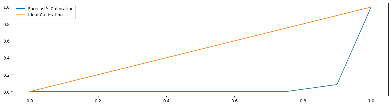
Often, the probabilistic forecast’s calibration is important. I.e., how many values are smaller then the 0.1 quantile, 0.2 quantile, etc.
This evaluation can be made using calibration plots:
[32]:
from sktime.utils.plotting import plot_calibration

plot_calibration(y_true=y_test.loc[pred_quantiles.index], y_pred=pred_quantiles)
[32]:
(<Figure size 1600x400 with 1 Axes>, <Axes: >)
Advanced composition: pipelines, tuning, reduction, adding proba forecasts to any estimator
composition = constructing “composite” estimators out of multiple “component” estimators
reduction = building estimator type A using estimator type B
special case: adding proba forecasting capability to non-proba forecaster
special case: using proba supervised learner for proba forecasting
pipelining = chaining estimators, here: transformers to a forecaster
tuning = automated hyper-parameter fitting, usually via internal evaluation loop
special case: grid parameter search and random parameter search tuning
special case: “Auto-ML”, optimizing not just estimator hyper-parameter but also choice of estimator
Adding probabilistic forecasts to non-probabilistic forecasters
start with a forecaster that does not produce probabilistic predictions:
[33]:
from sktime.forecasting.exp_smoothing import ExponentialSmoothing

my_forecaster = ExponentialSmoothing()

# does the forecaster support probabilistic predictions?
my_forecaster.get_tag("capability:pred_int")
[33]:
False
adding probabilistic predictions is possible via reduction wrappers:
[34]:
# NaiveVariance adds intervals & variance via collecting past residuals
from sktime.forecasting.naive import NaiveVariance

# create a composite forecaster like this:
my_forecaster_with_proba = NaiveVariance(my_forecaster)

# does it support probabilistic predictions now?
my_forecaster_with_proba.get_tag("capability:pred_int")
[34]:
True
the composite can now be used like any probabilistic forecaster:
[35]:
y = load_airline()

my_forecaster_with_proba.fit(y, fh=[1, 2, 3])
my_forecaster_with_proba.predict_interval()
[35]:
| Number of airline passengers | ||
|---|---|---|
| 0.9 | ||
| lower | upper | |
| 1961-01 | 341.960792 | 522.039207 |
| 1961-02 | 319.835453 | 544.164546 |
| 1961-03 | 307.334056 | 556.665943 |
roadmap items:
more compositors to enable probabilistic forecasting
bootstrap forecast intervals
reduction to probabilistic supervised learning
popular “add probabilistic capability” wrappers
contributions are appreciated!
Tuning and AutoML
ForecastingGridSearchCV or ForecastingRandomSearchCVchange metric to tune to a probabilistic metric
use a corresponding probabilistic metric or loss function
Internally, evaluation will be done using probabilistic metric, via backtesting evaluation.
evaluate or a separate benchmarking workflow.[36]:
from sktime.forecasting.model_selection import ForecastingGridSearchCV
from sktime.forecasting.theta import ThetaForecaster
from sktime.performance_metrics.forecasting.probabilistic import PinballLoss
from sktime.split import SlidingWindowSplitter

# forecaster we want to tune
forecaster = ThetaForecaster()

# parameter grid to search over
param_grid = {"sp": [1, 6, 12]}

# evaluation/backtesting regime for *tuning*
fh = [1, 2, 3]  # fh for tuning regime, does not need to be same as in fit/predict!
cv = SlidingWindowSplitter(window_length=36, fh=fh)
scoring = PinballLoss()

# construct the composite forecaster with grid search compositor
gscv = ForecastingGridSearchCV(
    forecaster, cv=cv, param_grid=param_grid, scoring=scoring, strategy="refit"
)
[37]:
from sktime.datasets import load_airline

y = load_airline()[:60]

gscv.fit(y, fh=fh)
[37]:
ForecastingGridSearchCV(cv=SlidingWindowSplitter(fh=[1, 2, 3],
                                                 window_length=36),
                        forecaster=ThetaForecaster(),
                        param_grid={'sp': [1, 6, 12]}, scoring=PinballLoss())
Please rerun this cell to show the HTML repr or trust the notebook.ForecastingGridSearchCV(cv=SlidingWindowSplitter(fh=[1, 2, 3],
window_length=36),
forecaster=ThetaForecaster(),
param_grid={'sp': [1, 6, 12]}, scoring=PinballLoss())SlidingWindowSplitter(fh=[1, 2, 3], window_length=36)
ThetaForecaster()
PinballLoss()
inspect hyper-parameter fit obtained by tuning:
[38]:
gscv.best_params_
[38]:
{'sp': 12}
obtain predictions:
[39]:
gscv.predict_interval()
[39]:
| Number of airline passengers | ||
|---|---|---|
| 0.9 | ||
| lower | upper | |
| 1954-01 | 190.832917 | 217.164705 |
| 1954-02 | 195.638436 | 226.620355 |
| 1954-03 | 221.947952 | 256.967883 |
for AutoML, use the MultiplexForecaster to select among multiple forecasters:
[40]:
from sktime.forecasting.compose import MultiplexForecaster
from sktime.forecasting.exp_smoothing import ExponentialSmoothing
from sktime.forecasting.naive import NaiveForecaster, NaiveVariance

forecaster = MultiplexForecaster(
    forecasters=[
        ("naive", NaiveForecaster(strategy="last")),
        ("ets", ExponentialSmoothing(trend="add", sp=12)),
    ],
)

forecaster_param_grid = {"selected_forecaster": ["ets", "naive"]}
gscv = ForecastingGridSearchCV(forecaster, cv=cv, param_grid=forecaster_param_grid)

gscv.fit(y)
gscv.best_params_
[40]:
{'selected_forecaster': 'naive'}
Pipelines with probabilistic forecasters
sktime pipelines are compatible with probabilistic forecasters:
ForecastingPipelineapplies transformers to the exogeneousXargument before passing them to the forecasterTransformedTargetForecastertransformsyand back-transforms forecasts, including interval or quantile forecasts
ForecastingPipeline takes a chain of transformers and forecasters, say,
[t1, t2, ..., tn, f],
where t[i] are forecasters that pre-process, and tp[i] are forecasters that postprocess
fit(y, X, fh) does:
X1 = t1.fit_transform(X)X2 = t2.fit_transform(X1)X[n] = t3.fit_transform(X[n-1])f.fit(y=y, x=X[n])
predict_[sth](X, fh) does:
X1 = t1.transform(X)X2 = t2.transform(X1)X[n] = t3.transform(X[n-1])f.predict_[sth](X=X[n], fh)
[41]:
from sktime.datasets import load_macroeconomic
from sktime.forecasting.arima import ARIMA
from sktime.forecasting.compose import ForecastingPipeline
from sktime.split import temporal_train_test_split
from sktime.transformations.impute import Imputer
[42]:
data = load_macroeconomic()
y = data["unemp"]
X = data.drop(columns=["unemp"])

y_train, y_test, X_train, X_test = temporal_train_test_split(y, X)
[43]:
forecaster = ForecastingPipeline(
    steps=[
        ("imputer", Imputer(method="mean")),
        ("forecaster", ARIMA(suppress_warnings=True)),
    ]
)
forecaster.fit(y=y_train, X=X_train, fh=X_test.index[:5])
forecaster.predict_interval(X=X_test[:5])
[43]:
| 0 | ||
|---|---|---|
| 0.9 | ||
| lower | upper | |
| Period | ||
| 1997Q1 | 5.042704 | 6.119990 |
| 1997Q2 | 3.948564 | 5.235163 |
| 1997Q3 | 3.887471 | 5.253592 |
| 1997Q4 | 4.108211 | 5.506862 |
| 1998Q1 | 4.501319 | 5.913611 |
TransformedTargetForecaster takes a chain of transformers and forecasters, say,
[t1, t2, ..., tn, f, tp1, tp2, ..., tk],
where t[i] are forecasters that pre-process, and tp[i] are forecasters that postprocess
fit(y, X, fh) does:
y1 = t1.fit_transform(y)y2 = t2.fit_transform(y1)y3 = t3.fit_transform(y2)y[n] = t3.fit_transform(y[n-1])f.fit(y[n])
yp1 = tp1.fit_transform(yn)yp2 = tp2.fit_transform(yp1)yp3 = tp3.fit_transform(yp2)predict_quantiles(y, X, fh) does:
y1 = t1.transform(y)y2 = t2.transform(y1)y[n] = t3.transform(y[n-1])y_pred = f.predict_quantiles(y[n])
y_pred = t[n].inverse_transform(y_pred)y_pred = t[n-1].inverse_transform(y_pred)y_pred = t1.inverse_transform(y_pred)y_pred = tp1.transform(y_pred)y_pred = tp2.transform(y_pred)y_pred = tp[n].transform(y_pred)Note: the remaining proba predictions are inferred from predict_quantiles.
[44]:
from sktime.datasets import load_macroeconomic
from sktime.forecasting.arima import ARIMA
from sktime.forecasting.compose import TransformedTargetForecaster
from sktime.transformations.detrend import Deseasonalizer, Detrender
[45]:
data = load_macroeconomic()
y = data[["unemp"]]
[46]:
forecaster = TransformedTargetForecaster(
    [
        ("deseasonalize", Deseasonalizer(sp=12)),
        ("detrend", Detrender()),
        ("forecast", ARIMA()),
    ]
)

forecaster.fit(y, fh=[1, 2, 3])
forecaster.predict_interval()
[46]:
| 0 | ||
|---|---|---|
| 0.9 | ||
| lower | upper | |
| 2009Q4 | 8.949103 | 10.068284 |
| 2010Q1 | 8.639806 | 10.206350 |
| 2010Q2 | 8.438112 | 10.337207 |
[47]:
forecaster.predict_quantiles()
[47]:
| 0 | ||
|---|---|---|
| 0.05 | 0.95 | |
| 2009Q4 | 8.949103 | 10.068284 |
| 2010Q1 | 8.639806 | 10.206350 |
| 2010Q2 | 8.438112 | 10.337207 |
quick creation also possible via the * dunder method, same pipeline:
[48]:
forecaster = Deseasonalizer(sp=12) * Detrender() * ARIMA()
[49]:
forecaster.fit(y, fh=[1, 2, 3])
forecaster.predict_interval()
[49]:
| 0 | ||
|---|---|---|
| 0.9 | ||
| lower | upper | |
| 2009Q4 | 8.949103 | 10.068284 |
| 2010Q1 | 8.639806 | 10.206350 |
| 2010Q2 | 8.438112 | 10.337207 |
Building your own probabilistic forecaster
Getting started:
follow the “implementing estimator” developer guide
use the advanced forecasting extension template
Extension template = python “fill-in” template with to-do blocks that allow you to implement your own, sktime-compatible forecasting algorithm.
Check estimators using check_estimator
For probabilistic forecasting:
implement at least one of
predict_quantiles,predict_interval,predict_var,predict_probaoptimally, implement all, unless identical with defaulting behaviour as below
if only one is implemented, others use following defaults (in this sequence, dependent availability):
predict_intervaluses quantiles frompredict_quantilesand vice versapredict_varuses variance frompredict_proba, or variance of normal with IQR as obtained frompredict_quantilespredict_intervalorpredict_quantilesuses quantiles frompredict_probadistributionpredict_probareturns normal with meanpredictand variancepredict_var
so if predictive residuals not normal, implement
predict_probaorpredict_quantilesif interfacing, implement the ones where least “conversion” is necessary
ensure to set the
capability:pred_inttag toTrue
[50]:
# estimator checking on the fly using check_estimator

# suppose NaiveForecaster is your new estimator
from sktime.forecasting.naive import NaiveForecaster

# check the estimator like this

# uncomment this block to run

# from sktime.utils.estimator_checks import check_estimator
#
# check_estimator(NaiveForecaster)

# this prints any failed tests, and returns dictionary with
#   keys of test runs and results from the test run
# run individual tests using the tests_to_run arg or the fixtures_to_run_arg
#   these need to be identical to test or test/fixture names, see docstring
[51]:
# to raise errors for use in traceback debugging:

# uncomment next line to run
# check_estimator(NaiveForecaster, raise_exceptions=True)

# this does not raise an error since NaiveForecaster is fine, but would if it weren't
Summary
unified API for probabilistic forecasting and probabilistic metrics
integrating other packages (e.g. scikit-learn, statsmodels, pmdarima, prophet)
interface for composite model building is same, proba or not (pipelining, ensembling, tuning, reduction)
easily extensible with custom estimators
Useful resources
For more details, take a look at our paper on forecasting with sktime in which we discuss the forecasting API in more detail and use it to replicate and extend the M4 study.
For a good introduction to forecasting, see Hyndman, Rob J., and George Athanasopoulos. Forecasting: principles and practice. OTexts, 2018.
For comparative benchmarking studies/forecasting competitions, see the M4 competition and the M5 competition.
Credits
notebook creation: fkiraly
Generated using nbsphinx. The Jupyter notebook can be found here.