Exercise

Exercise

[1]:

# !pip install cointanalysis matplotlib numpy pandas pandas_datareader scipy seaborn sklearn statsmodels  # noqa: E501
# !pip install fracdiff

[2]:

import matplotlib.pyplot as plt
import numpy as np
import pandas as pd
import pandas_datareader
import seaborn
from fracdiff import Fracdiff, FracdiffStat, fdiff
from statsmodels.tsa.stattools import adfuller

seaborn.set_style("white")

[3]:

def adf_test(array):
    """Carry out ADF unit-root test and print the result."""
    adf, pvalue, _, _, _, _ = adfuller(array)
    print(f"* ADF statistics: {adf:.3f}")
    print(f"* ADF p-value: {pvalue:.3f}")

5.1

• Prepare Gaussian, its cumsum and its differentiation.

[4]:

np.random.seed(42)
gauss = np.random.randn(1000)
brown = gauss.cumsum()
overd = np.diff(gauss)

[5]:

plt.figure(figsize=(24, 6))

plt.subplot(1, 3, 1)
plt.plot(gauss, lw=0.6)
plt.title("gauss")

plt.subplot(1, 3, 2)
plt.plot(brown, lw=0.6)
plt.title("brown")

plt.subplot(1, 3, 3)
plt.plot(overd, lw=0.6)
plt.title("over-differentiated")

plt.show()

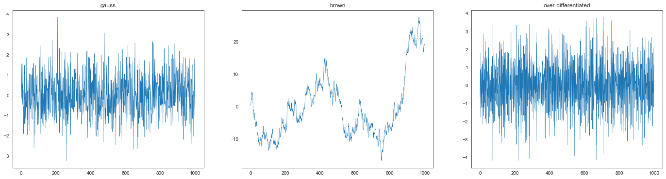
5.1 (a)

[6]:

adf_test(gauss)

* ADF statistics: -31.811
* ADF p-value: 0.000

5.1 (b)

• Order of integration of cumsum is 1.

[7]:

adf_test(brown)

* ADF statistics: -0.966
* ADF p-value: 0.765

5.1 (c)

• ADF statistics and p-value of over-differentiated process are:

[8]:

adf_test(overd)

* ADF statistics: -11.486
* ADF p-value: 0.000

5.2

• Prepare sin function and the process given by (sin + shift).cumsum() (which we call hop):

[9]:

sin = np.sin(np.linspace(0, 10 * np.pi, 1000))
hop = (sin + 0.1).cumsum()

[10]:

plt.figure(figsize=(24, 6))

plt.subplot(1, 2, 1)
plt.title("sin")
plt.plot(sin)

plt.subplot(1, 2, 2)
plt.title("hop")
plt.plot(hop)

plt.show()

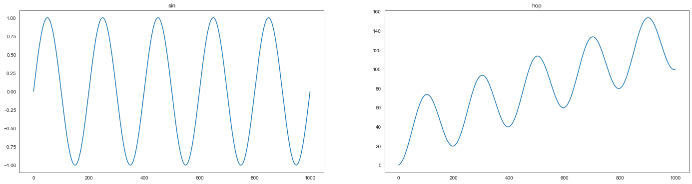
5.2 (a)

[11]:

adf_test(sin)

* ADF statistics: -13323341825676.293
* ADF p-value: 0.000

5.2 (b)

[12]:

adf_test(hop)

* ADF statistics: -0.284
* ADF p-value: 0.928

• Let us see ADF p-values of fracdiff of hop with various orders:

• Notice: We will use the fixed-window method instead of expanding window method.

[13]:

ds = (
    0.200,
    0.400,
    0.600,
    0.800,
    0.900,
    0.990,
    0.999,
    1.000,
)
window = 100

X = hop.reshape(-1, 1)

plt.figure(figsize=(24, 8))
for i, d in enumerate(ds):
    diff = fdiff(hop, d, window=window)
    _, pvalue, _, _, _, _ = adfuller(diff)

    plt.subplot(2, 4, i + 1)
    plt.title(f"hop, {d:.3f} th diff (p={pvalue:.2f})")
    plt.plot(diff)

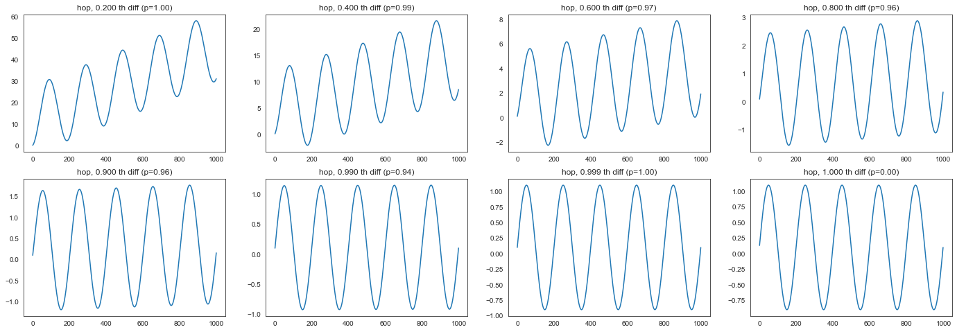
• It seems that the minimum order is pretty close to 1.0.

• Let us search the minimum using FracdiffStat.

[14]:

precision = 10e-8

f = FracdiffStat(window=window, mode="valid", precision=precision, lower=0.9)

diff = f.fit_transform(X)

print(f"* Order: {f.d_[0]:.8f}")
adf_test(diff)

* Order: 0.99999971
* ADF statistics: -280803737.580
* ADF p-value: 0.000

[16]:

# Check

diff = Fracdiff(f.d_[0] - precision, mode="valid").fit_transform(X)

print(f"* Order: {f.d_[0] - precision:.8f}")
adf_test(diff)

* Order: 0.99999961
* ADF statistics: 0.001
* ADF p-value: 0.959

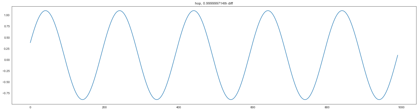
• Differentiated time-series looks like this:

[17]:

plt.figure(figsize=(24, 6))
plt.plot(diff)
plt.title(f"hop, {f.d_[0]:.9f}th diff")
plt.show()

5.3

5.3 (a)

[18]:

from sklearn.linear_model import LinearRegression

[19]:

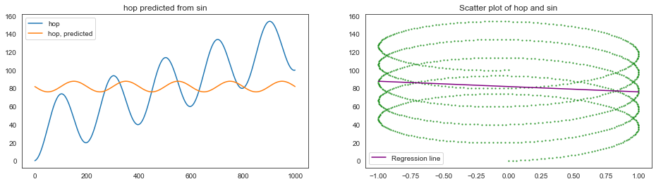
linreg = LinearRegression()
linreg.fit(sin.reshape(-1, 1), hop)

print(f"* R-squared: {linreg.score(sin.reshape(-1, 1), hop):.4f}")

* R-squared: 0.0128

[20]:

plt.figure(figsize=(16, 4))

plt.subplot(1, 2, 1)
plt.title("hop predicted from sin")
plt.plot(hop, label="hop")
plt.plot(linreg.predict(sin.reshape(-1, 1)), label="hop, predicted")
plt.legend()

plt.subplot(1, 2, 2)
plt.title("Scatter plot of hop and sin")
x = np.linspace(-1, 1, 2)
y = linreg.predict(x.reshape(-1, 1))
plt.scatter(sin, hop, s=2, alpha=0.6, color="green")
plt.plot(x, y, color="purple", label="Regression line")
plt.legend()

plt.show()

5.3 (b)

[21]:

hopd = np.diff(hop)

linreg = LinearRegression()
linreg.fit(sin[1:].reshape(-1, 1), hopd)

print(f"* Coefficient: {linreg.coef_[0]}")
print(f"* Intercept: {linreg.intercept_}")
print(f"* R-squared: {linreg.score(sin[1:].reshape(-1, 1), hopd):.4f}")

* Coefficient: 0.9999999999999994
* Intercept: 0.1
* R-squared: 1.0000

5.3 (c)

• d=1. Because 1st order differentiation of hop is sin plus a constant.

5.4

• NOTE: We will use time-bar instead of dollar-bar.

[22]:

def fetch_spx(begin="1998-01-01", end="2020-09-30"):  # noqa: D103
    return pandas_datareader.data.DataReader("^GSPC", "yahoo", begin, end)["Adj Close"]

[23]:

spx = fetch_spx()

[24]:

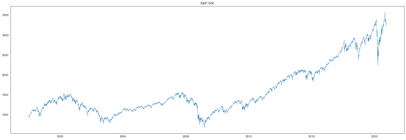
plt.figure(figsize=(24, 8))
plt.plot(spx, linewidth=0.6)
plt.title("S&P 500")
plt.show()

[25]:

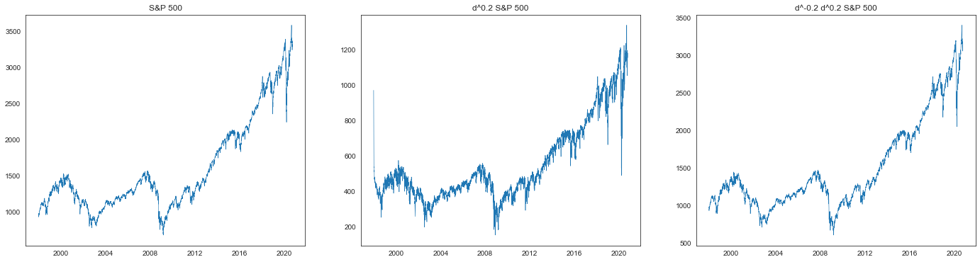
d = 0.2
window = 100

d0 = fdiff(spx.values, d, window=window, mode="full")
d1 = fdiff(d0, -d, window=window, mode="full")

spxd = pd.Series(d0, index=spx.index)
spxi = pd.Series(d1, index=spx.index)

• What we get is, in principle, the original time-series plus some constant.

• While there are small numerical errors due to the cut-off of a sequence of coefficients with a finite window.

[26]:

plt.figure(figsize=(24, 6))

plt.subplot(1, 3, 1)
plt.title("S&P 500")
plt.plot(spx, linewidth=0.6)

plt.subplot(1, 3, 2)
plt.title(f"d^{d} S&P 500")
plt.plot(spxd, linewidth=0.6)

plt.subplot(1, 3, 3)
plt.title(f"d^{-d} d^{d} S&P 500")
plt.plot(spxi, linewidth=0.6)

plt.show()

5.5

5.5 (a)

[27]:

spxlog = spx.apply(np.log)

spxlogcumsum = spxlog.cumsum()
spxlogcumsum

[27]:

Date
1997-12-31        6.877739
1998-01-02       13.760218
1998-01-05       20.644776
1998-01-06       27.518540
1998-01-07       34.389631
                  ...
2020-09-24    41792.094032
2020-09-25    41800.195243
2020-09-28    41808.312436
2020-09-29    41816.424805
2020-09-30    41824.545394
Name: Adj Close, Length: 5725, dtype: float64

5.5 (b)

[28]:

from fracdiff.tol import window_from_tol_coef

window = window_from_tol_coef(0.5, 1e-5)
window

[28]:

928

[29]:

X = np.array(spxlogcumsum).reshape(-1, 1)

f = FracdiffStat(window=window, mode="valid", upper=2)
diff = f.fit_transform(X)

print(f"* Order: {f.d_[0]:.2f}")

* Order: 1.73

[30]:

# Check stationarity
adf_test(diff)

* ADF statistics: -2.868
* ADF p-value: 0.049

5.5 (c)

[31]:

X = spxlog.values.reshape(-1, 1)

f = FracdiffStat(window=window, mode="valid")
spxlogd = pd.Series(f.fit_transform(X).reshape(-1), index=spx.index[-diff.size :])

[32]:

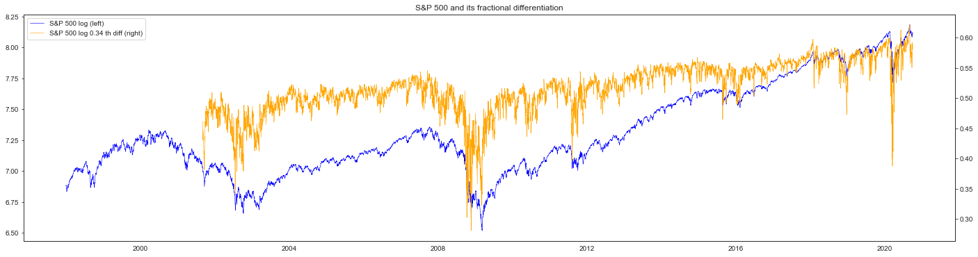
corr = np.corrcoef(spxlog[-spxd.size :], spxd)[0, 1]

print(f"* Correlation: {corr:.2f}")

* Correlation: 0.98

[33]:

fig, ax_s = plt.subplots(figsize=(24, 6))
ax_d = ax_s.twinx()

plot_s = ax_s.plot(
    spxlog[-spxd.size :], color="blue", linewidth=0.6, label="S&P 500 log (left)"
)
plot_d = ax_d.plot(
    spxlogd,
    color="orange",
    linewidth=0.6,
    label=f"S&P 500 log {f.d_[0]:.2f} th diff (right)",
)
plots = plot_s + plot_d

plt.title("S&P 500 and its fractional differentiation")
ax_s.legend(plots, [p.get_label() for p in plots], loc=0)

plt.show()

5.5 (d)

[34]:

from cointanalysis import CointAnalysis

• It is nonsense to discuss cointegration of Xd because cointegration is defined among non-stationary processes and Xd is stationary.

• So we will instead discuss cointegration between 1.3 th differentiated time-series, which is non-stationary, with the original time-series.

[35]:

d = 0.30

# Check non-stationarity
diff = fdiff(spxlog, d, window=window, mode="valid")
spxlogd = pd.Series(diff, index=spxlog.index[-diff.size :])
adf_test(diff)

* ADF statistics: -2.445
* ADF p-value: 0.129

[36]:

pair = np.stack((spxlog[-diff.size :], diff), 1)

ca = CointAnalysis().test(pair)

print(f"* AEG statistics: {ca.stat_:.2f}")
print(f"* AEG p-value: {ca.pvalue_:.2e}")

* AEG statistics: -4.26
* AEG p-value: 2.96e-03

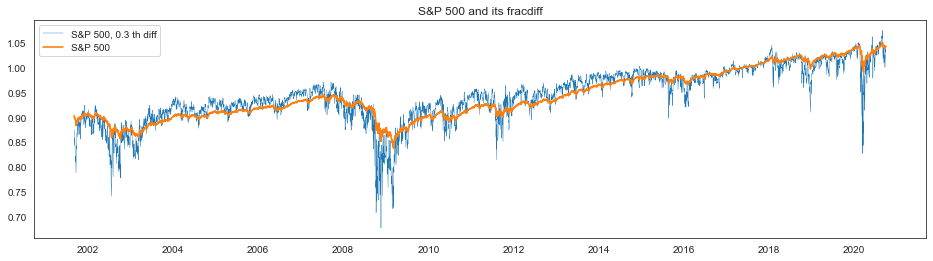
• They are cointegrated.

• Rough reason: For d=0, two series are exactly the same and so trivially cointegrated. For d that is close to the minimum value to make fracdiff stationary, one can make an almost stationary series by adding the original series multiplied by an infinitesimally small coefficient to fracdiff. One can expect cointegration for any d in between assuming an interpolation.

[37]:

ca.fit(pair)

ys = (-spxlog * ca.coef_[0])[-spxlogd.size :]
yd = spxlogd * ca.coef_[1] - ca.mean_

[38]:

plt.figure(figsize=(16, 4))

plt.plot(yd, linewidth=0.4, label=f"S&P 500, {d} th diff")
plt.plot(ys, linewidth=1.6, label="S&P 500")

plt.legend()
plt.title("S&P 500 and its fracdiff")
plt.show()

[39]:

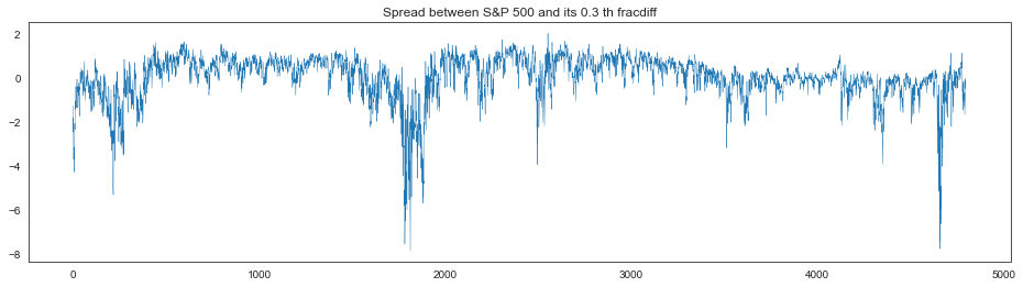
spread = ca.transform(pair)

[40]:

plt.figure(figsize=(16, 4))
plt.plot(spread, linewidth=0.4)
plt.title(f"Spread between S&P 500 and its {d} th fracdiff")
plt.show()

5.5 (e)

[41]:

from statsmodels.stats.stattools import jarque_bera

[42]:

spxlogd.values.reshape(-1, 1).shape

[42]:

(4798, 1)

[43]:

X = spxlog.values.reshape(-1, 1)

f = FracdiffStat(window=window, mode="valid")
spxlogd = pd.Series(f.fit_transform(X).reshape(-1), index=spx.index[-diff.size :])

spxlr = spxlog.diff()[-spxlogd.size :]  # logreturn

pd.DataFrame(
    {
        "S&P 500": jarque_bera(spx[-spxlogd.size :]),
        "S&P 500 fracdiff": jarque_bera(spxlogd),
        "S&P 500 logreturn": jarque_bera(spxlr),
    },
    index=["JB statistics", "p-value", "skew", "kurtosis"],
).round(3)

[43]:

	S&P 500	S&P 500 fracdiff	S&P 500 logreturn
JB statistics	637.418	1110.285	29941.995
p-value	0.000	0.000	0.000
skew	0.873	-0.834	-0.445
kurtosis	2.629	4.664	15.206

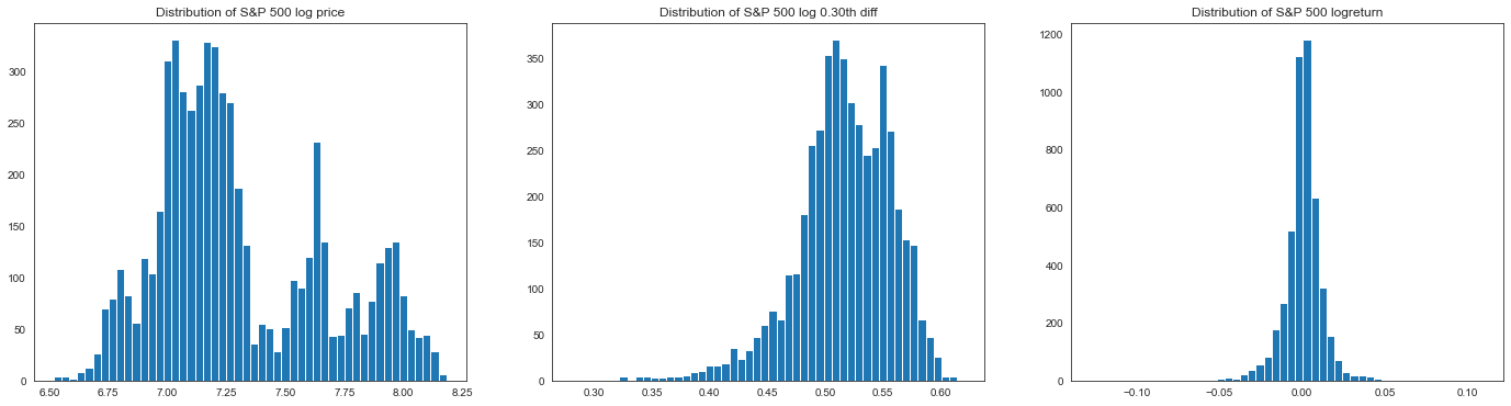
[44]:

plt.figure(figsize=(24, 6))

plt.subplot(1, 3, 1)
plt.title("Distribution of S&P 500 log price")
plt.hist(spxlog, bins=50)

plt.subplot(1, 3, 2)
plt.title(f"Distribution of S&P 500 log {d:.2f}th diff")
plt.hist(spxlogd, bins=50)

plt.subplot(1, 3, 3)
plt.title("Distribution of S&P 500 logreturn")
plt.hist(spxlr, bins=50)

plt.show()

[ ]:

---

Generated using nbsphinx. The Jupyter notebook can be found here.