![]()
Set-up instructions: this notebook give a tutorial on the forecasting learning task supported by sktime. On binder, this should run out-of-the-box.
To run this notebook as intended, ensure that sktime with basic dependency requirements is installed in your python environment.
To run this notebook with a local development version of sktime, an editable developer installation is recommended, see the sktime developer install guide for instructions.
Forecasting with sktime#
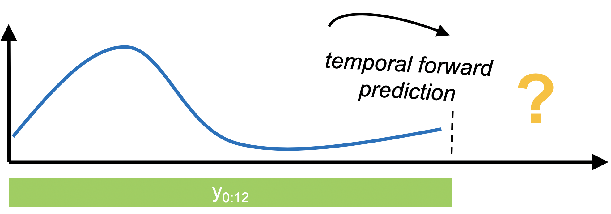
In forecasting, past data is used to make temporal forward predictions of a time series. This is notably different from tabular prediction tasks supported by scikit-learn and similar libraries.
sktime provides a common, scikit-learn-like interface to a variety of classical and ML-style forecasting algorithms, together with tools for building pipelines and composite machine learning models, including temporal tuning schemes, or reductions such as walk-forward application of scikit-learn regressors.
Section 1 provides an overview of common forecasting workflows supported by sktime.
Section 2 discusses the families of forecasters available in sktime.
Section 3 discusses advanced composition patterns, including pipeline building, reduction, tuning, ensembling, and autoML.
Section 4 gives an introduction to how to write custom estimators compliant with the sktime interface.
Further references: * For further details on how forecasting is different from supervised prediction à la scikit-learn, and pitfalls of misdiagnosing forecasting as supervised prediction, have a look at this notebook * For a scientific reference, take a look at our paper on forecasting with sktime in which we discuss sktime’s forecasting module in more detail and use it to replicate and extend the M4 study.
Table of Contents#
1. Basic forecasting workflows
1.1 Data container format
1.2 Basic deployment workflow - batch fitting and forecasting
1.2.1 Basic deployment workflow in a nutshell
1.2.2 Forecasters that require the horizon when fitting
1.2.3 Forecasters that can make use of exogeneous data
1.2.4 Multivariate Forecasters
1.2.5 Prediction intervals and quantile forecasts
1.2.6 Panel forecasts and hierarchical forecasts
1.3 Basic evaluation workflow - evaluating a batch of forecasts against ground truth observations
1.3.1 The basic batch forecast evaluation workflow in a nutshell - function metric interface
1.3.2 The basic batch forecast evaluation workflow in a nutshell - metric class interface
1.4 Advanced deployment workflow: rolling updates & forecasts
1.4.1 Updating a forecaster with the update method
1.4.2 Moving the “now” state without updating the model
1.4.3 Walk-forward predictions on a batch of data
1.5 Advanced evaluation workflow: rolling re-sampling and aggregate errors, rolling back-testing
2. Forecasters in sktime - searching, tags, common families
2.1 Forecaster lookup - the registry
2.2 Forecaster tags
2.2.1 Capability tags: multivariate, probabilistic, hierarchical
2.2.2 Finding and listing forecasters by tag
2.2.3 Listing all forecaster tags
2.3 Common forecaster types
2.3.1 Exponential smoothing, theta forecaster, autoETS from statsmodels
2.3.2 ARIMA and autoARIMA
2.3.3 BATS and TBATS
2.3.4 Facebook prophet
2.3.5 State Space Model (Structural Time Series)
2.3.6 AutoArima from StatsForecast
3. Advanced composition patterns - pipelines, reduction, autoML, and more
3.1 Reduction: from forecasting to regression
3.2 Pipelining, detrending and deseasonalization
3.2.1 The basic forecasting pipeline
3.2.2 The Detrender as pipeline component
3.2.3 Complex pipeline composites and parameter inspection
3.3 Parameter tuning
3.3.1 Basic tuning using ForecastingGridSearchCV
3.3.2 Tuning of complex composites
3.3.3 Selecting the metric and retrieving scores
3.4 autoML aka automated model selection, ensembling and hedging
3.4.1 autoML aka automatic model selection, using tuning plus multiplexer
3.4.2 autoML: selecting transformer combinations via OptimalPassthrough
3.4.3 Simple ensembling strategies
3.4.4 Prediction weighted ensembles and hedge ensembles
4. Extension guide - implementing your own forecaster
5. Summary
Package imports#
[1]:
import warnings

import numpy as np
import pandas as pd

# hide warnings
warnings.filterwarnings("ignore")
1. Basic forecasting workflows#
This section explains the basic forecasting workflows, and key interface points for it.
We cover the following four workflows:
Basic deployment workflow: batch fitting and forecasting
Basic evaluation workflow: evaluating a batch of forecasts against ground truth observations
Advanced deployment workflow: fitting and rolling updates/forecasts
Advanced evaluation workflow: using rolling forecast splits and computing split-wise and aggregate errors, including common back-testing schemes
All workflows make common assumptions on the input data format.
sktime uses pandas for representing time series:
pd.DataFramefor time series and sequences, primarily. Rows represent time indices, columns represent variables.pd.Seriescan also be used for univariate time series and sequencesnumpyarrays (1D and 2D) can also be passed, butpandasuse is encouraged.
The Series.index and DataFrame.index are used for representing the time series or sequence index. sktime supports pandas integer, period and timestamp indices for simple time series.
sktime supports further, additional container formats for panel and hierarchical time series, these are discussed in Section 1.6.
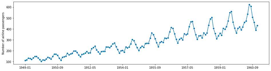
Example: as the running example in this tutorial, we use a textbook data set, the Box-Jenkins airline data set, which consists of the number of monthly totals of international airline passengers, from 1949 - 1960. Values are in thousands. See “Makridakis, Wheelwright and Hyndman (1998) Forecasting: methods and applications”, exercises sections 2 and 3.
[2]:
from sktime.datasets import load_airline
from sktime.utils.plotting import plot_series
[3]:
y = load_airline()

# plotting for visualization
plot_series(y)
[3]:
(<Figure size 1152x288 with 1 Axes>,
 <AxesSubplot:ylabel='Number of airline passengers'>)
[4]:
y.index
[4]:
PeriodIndex(['1949-01', '1949-02', '1949-03', '1949-04', '1949-05', '1949-06',
             '1949-07', '1949-08', '1949-09', '1949-10',
             ...
             '1960-03', '1960-04', '1960-05', '1960-06', '1960-07', '1960-08',
             '1960-09', '1960-10', '1960-11', '1960-12'],
            dtype='period[M]', length=144)
Generally, users are expected to use the in-built loading functionality of pandas and pandas-compatible packages to load data sets for forecasting, such as read_csv or the Series or DataFrame constructors if data is available in another in-memory format, e.g., numpy.array.
sktime forecasters may accept input in pandas-adjacent formats, but will produce outputs in, and attempt to coerce inputs to, pandas formats.
NOTE: if your favourite format is not properly converted or coerced, kindly consider to contribute that functionality to sktime.
The simplest use case workflow is batch fitting and forecasting, i.e., fitting a forecasting model to one batch of past data, then asking for forecasts at time point in the future.
The steps in this workflow are as follows:
Preparation of the data
Specification of the time points for which forecasts are requested. This uses a
numpy.arrayor theForecastingHorizonobject.Specification and instantiation of the forecaster. This follows a
scikit-learn-like syntax; forecaster objects follow the familiarscikit-learnBaseEstimatorinterface.Fitting the forecaster to the data, using the forecaster’s
fitmethodMaking a forecast, using the forecaster’s
predictmethod
The below first outlines the vanilla variant of the basic deployment workflow, step-by-step.
At the end, one-cell workflows are provided, with common deviations from the pattern (Sections 1.2.1 and following).
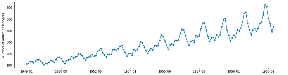
Step 1 - Preparation of the data#
As discussed in Section 1.1, the data is assumed to be in pd.Series or pd.DataFrame format.
[5]:
from sktime.datasets import load_airline
from sktime.utils.plotting import plot_series
[6]:
# in the example, we use the airline data set.
y = load_airline()
plot_series(y)
[6]:
(<Figure size 1152x288 with 1 Axes>,
 <AxesSubplot:ylabel='Number of airline passengers'>)
Step 2 - Specifying the forecasting horizon#
Now we need to specify the forecasting horizon and pass that to our forecasting algorithm.
There are two main ways:
Using a
numpy.arrayof integers. This assumes either integer index or periodic index (PeriodIndex) in the time series; the integer indicates the number of time points or periods ahead we want to make a forecast for. E.g.,1means forecast the next period,2the second next period, and so on.Using a
ForecastingHorizonobject. This can be used to define forecast horizons, using any supported index type as an argument. No periodic index is assumed.
Forecasting horizons can be absolute, i.e., referencing specific time points in the future, or relative, i.e., referencing time differences to the present. As a default, the present is that latest time point seen in any y passed to the forecaster.
numpy.array based forecasting horizons are always relative; ForecastingHorizon objects can be both relative and absolute. In particular, absolute forecasting horizons can only be specified using ForecastingHorizon.
Using a numpy forecasting horizon#
[7]:
fh = np.arange(1, 37)
fh
[7]:
array([ 1,  2,  3,  4,  5,  6,  7,  8,  9, 10, 11, 12, 13, 14, 15, 16, 17,
       18, 19, 20, 21, 22, 23, 24, 25, 26, 27, 28, 29, 30, 31, 32, 33, 34,
       35, 36])
This will ask for monthly predictions for the next three years, since the original series period is 1 month. In another example, to predict only the second and fifth month ahead, one could write:
import numpy as np
fh = np.array([2, 5])  # 2nd and 5th step ahead
Using a ForecastingHorizon based forecasting horizon#
The ForecastingHorizon object takes absolute indices as input, but considers the input absolute or relative depending on the is_relative flag.
ForecastingHorizon will automatically assume a relative horizon if temporal difference types from pandas are passed; if value types from pandas are passed, it will assume an absolute horizon.
To define an absolute ForecastingHorizon in our example:
[8]:
from sktime.forecasting.base import ForecastingHorizon
[9]:
fh = ForecastingHorizon(
    pd.PeriodIndex(pd.date_range("1961-01", periods=36, freq="M")), is_relative=False
)
fh
[9]:
ForecastingHorizon(['1961-01', '1961-02', '1961-03', '1961-04', '1961-05', '1961-06',
             '1961-07', '1961-08', '1961-09', '1961-10', '1961-11', '1961-12',
             '1962-01', '1962-02', '1962-03', '1962-04', '1962-05', '1962-06',
             '1962-07', '1962-08', '1962-09', '1962-10', '1962-11', '1962-12',
             '1963-01', '1963-02', '1963-03', '1963-04', '1963-05', '1963-06',
             '1963-07', '1963-08', '1963-09', '1963-10', '1963-11', '1963-12'],
            dtype='period[M]', is_relative=False)
ForecastingHorizon-s can be converted from relative to absolute and back via the to_relative and to_absolute methods. Both of these conversions require a compatible cutoff to be passed:
[10]:
cutoff = pd.Period("1960-12", freq="M")
[11]:
fh.to_relative(cutoff)
[11]:
ForecastingHorizon([ 1,  2,  3,  4,  5,  6,  7,  8,  9, 10, 11, 12, 13, 14, 15, 16, 17,
            18, 19, 20, 21, 22, 23, 24, 25, 26, 27, 28, 29, 30, 31, 32, 33, 34,
            35, 36],
           dtype='int64', is_relative=True)
[12]:
fh.to_absolute(cutoff)
[12]:
ForecastingHorizon(['1961-01', '1961-02', '1961-03', '1961-04', '1961-05', '1961-06',
             '1961-07', '1961-08', '1961-09', '1961-10', '1961-11', '1961-12',
             '1962-01', '1962-02', '1962-03', '1962-04', '1962-05', '1962-06',
             '1962-07', '1962-08', '1962-09', '1962-10', '1962-11', '1962-12',
             '1963-01', '1963-02', '1963-03', '1963-04', '1963-05', '1963-06',
             '1963-07', '1963-08', '1963-09', '1963-10', '1963-11', '1963-12'],
            dtype='period[M]', is_relative=False)
Step 3 - Specifying the forecasting algorithm#
To make forecasts, a forecasting algorithm needs to be specified. This is done using a scikit-learn-like interface. Most importantly, all sktime forecasters follow the same interface, so the preceding and remaining steps are the same, no matter which forecaster is being chosen.
For this example, we choose the naive forecasting method of predicting the last seen value. More complex specifications are possible, using pipeline and reduction construction syntax; this will be covered later in Section 2.
[13]:
from sktime.forecasting.naive import NaiveForecaster
[14]:
forecaster = NaiveForecaster(strategy="last")
Step 4 - Fitting the forecaster to the seen data#
Now the forecaster needs to be fitted to the seen data:
[15]:
forecaster.fit(y)
[15]:
NaiveForecaster()
Step 5 - Requesting forecasts#
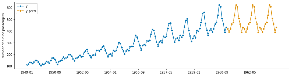
Finally, we request forecasts for the specified forecasting horizon. This needs to be done after fitting the forecaster:
[16]:
y_pred = forecaster.predict(fh)
[17]:
# plotting predictions and past data
plot_series(y, y_pred, labels=["y", "y_pred"])
[17]:
(<Figure size 1152x288 with 1 Axes>,
 <AxesSubplot:ylabel='Number of airline passengers'>)
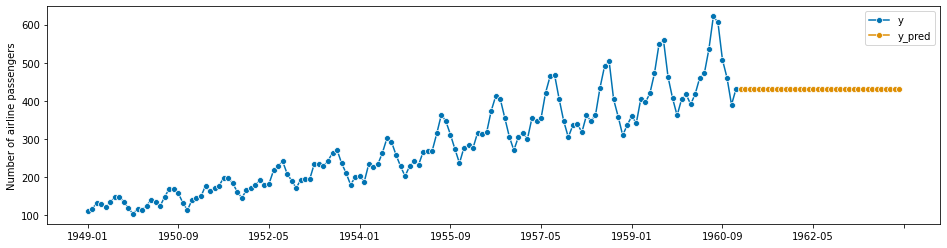
1.2.1 The basic deployment workflow in a nutshell#
For convenience, we present the basic deployment workflow in one cell. This uses the same data, but different forecaster: predicting the latest value observed in the same month.
[18]:
from sktime.datasets import load_airline
from sktime.forecasting.base import ForecastingHorizon
from sktime.forecasting.naive import NaiveForecaster
[19]:
# step 1: data specification
y = load_airline()

# step 2: specifying forecasting horizon
fh = np.arange(1, 37)

# step 3: specifying the forecasting algorithm
forecaster = NaiveForecaster(strategy="last", sp=12)

# step 4: fitting the forecaster
forecaster.fit(y)

# step 5: querying predictions
y_pred = forecaster.predict(fh)
[20]:
# optional: plotting predictions and past data
plot_series(y, y_pred, labels=["y", "y_pred"])
[20]:
(<Figure size 1152x288 with 1 Axes>,
 <AxesSubplot:ylabel='Number of airline passengers'>)
1.2.2 Forecasters that require the horizon already in fit#
Some forecasters need the forecasting horizon provided already in fit. Such forecasters will produce informative error messages when it is not passed in fit. All forecaster will remember the horizon when already passed in fit for prediction. The modified workflow to allow for such forecasters in addition is as follows:
[21]:
# step 1: data specification
y = load_airline()

# step 2: specifying forecasting horizon
fh = np.arange(1, 37)

# step 3: specifying the forecasting algorithm
forecaster = NaiveForecaster(strategy="last", sp=12)

# step 4: fitting the forecaster
forecaster.fit(y, fh=fh)

# step 5: querying predictions
y_pred = forecaster.predict()
1.2.3 Forecasters that can make use of exogeneous data#
Many forecasters can make use of exogeneous time series, i.e., other time series that are not forecast, but are useful for forecasting y. Exogeneous time series are always passed as an X argument, in fit, predict, and other methods (see below). Exogeneous time series should always be passed as pandas.DataFrames. Most forecasters that can deal with exogeneous time series will assume that the time indices of X passed to fit are a super-set of the time indices in y
passed to fit; and that the time indices of X passed to predict are a super-set of time indices in fh, although this is not a general interface restriction. Forecasters that do not make use of exogeneous time series still accept the argument (and do not use it internally).
The general workflow for passing exogeneous data is as follows:
[22]:
# step 1: data specification
y = load_airline()
# we create some dummy exogeneous data
X = pd.DataFrame(index=y.index)

# step 2: specifying forecasting horizon
fh = np.arange(1, 37)

# step 3: specifying the forecasting algorithm
forecaster = NaiveForecaster(strategy="last", sp=12)

# step 4: fitting the forecaster
forecaster.fit(y, X=X, fh=fh)

# step 5: querying predictions
y_pred = forecaster.predict(X=X)
NOTE: as in workflows 1.2.1 and 1.2.2, some forecasters that use exogeneous variables may also require the forecasting horizon only in predict. Such forecasters may also be called with steps 4 and 5 being
forecaster.fit(y, X=X)
y_pred = forecaster.predict(fh=fh, X=X)
1.2.4. Multivariate forecasting#
All forecasters in sktime support multivariate forecasts - some forecasters are “genuine” multivariate, all others “apply by column”.
Below is an example of the general multivariate forecasting workflow, using the VAR (vector auto-regression) forecaster on the Longley dataset from sktime.datasets. The workflow is the same as in the univariate forecasters, but the input has more than one variables (columns).
[23]:
from sktime.datasets import load_longley
from sktime.forecasting.var import VAR

_, y = load_longley()

y = y.drop(columns=["UNEMP", "ARMED", "POP"])

forecaster = VAR()
forecaster.fit(y, fh=[1, 2, 3])

y_pred = forecaster.predict()
The input to the multivariate forecaster y is a pandas.DataFrame where each column is a variable.
[24]:
y
[24]:
| GNPDEFL | GNP | |
|---|---|---|
| Period | ||
| 1947 | 83.0 | 234289.0 |
| 1948 | 88.5 | 259426.0 |
| 1949 | 88.2 | 258054.0 |
| 1950 | 89.5 | 284599.0 |
| 1951 | 96.2 | 328975.0 |
| 1952 | 98.1 | 346999.0 |
| 1953 | 99.0 | 365385.0 |
| 1954 | 100.0 | 363112.0 |
| 1955 | 101.2 | 397469.0 |
| 1956 | 104.6 | 419180.0 |
| 1957 | 108.4 | 442769.0 |
| 1958 | 110.8 | 444546.0 |
| 1959 | 112.6 | 482704.0 |
| 1960 | 114.2 | 502601.0 |
| 1961 | 115.7 | 518173.0 |
| 1962 | 116.9 | 554894.0 |
The result of the multivariate forecaster y_pred is a pandas.DataFrame where columns are the predicted values for each variable. The variables in y_pred are the same as in y, the input to the multivariate forecaster.
[25]:
y_pred
[25]:
| GNPDEFL | GNP | |
|---|---|---|
| 1963 | 121.688295 | 578514.398653 |
| 1964 | 124.353664 | 601873.015890 |
| 1965 | 126.847886 | 625411.588754 |
As said above, all forecasters accept multivariate input and will produce multivariate forecasts. There are two categories:
forecasters that are genuinely multivariate, such as
VAR. Forecasts for one endogeneous (y) variable will depend on values of other variables.forecasters that are univariate, such as
ARIMA. Forecasts will be made by endogeneous (y) variable, and not be affected by other variables.
To display complete list of multivariate forecasters, search for forecasters with 'multivariate' or 'both' tag value for the tag 'scitype:y', as follows:
[26]:
from sktime.registry import all_estimators

for forecaster in all_estimators(filter_tags={"scitype:y": ["multivariate", "both"]}):
    print(forecaster[0])
Univariate forecasters have tag value 'univariate', and will fit one model per column. To access the column-wise models, access the forecasters_ parameter, which stores the fitted forecasters in a pandas.DataFrame, fitted forecasters being in the column with the variable for which the forecast is being made:
[27]:
from sktime.datasets import load_longley
from sktime.forecasting.arima import ARIMA

_, y = load_longley()

y = y.drop(columns=["UNEMP", "ARMED", "POP"])

forecaster = ARIMA()
forecaster.fit(y, fh=[1, 2, 3])

forecaster.forecasters_
[27]:
| GNPDEFL | GNP | |
|---|---|---|
| forecasters | ARIMA() | ARIMA() |
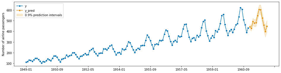
1.2.5 Probabilistic forecasting: prediction intervals, quantile, variance, and distributional forecasts#
sktime provides a unified interface to make probabilistic forecasts. The following methods are possibly available for probabilistic forecasts:
predict_intervalproduces interval forecasts. Additionally to anypredictarguments, an argumentcoverage(nominal interval coverage) must be provided.predict_quantilesproduces quantile forecasts. Additionally to anypredictarguments, an argumentalpha(quantile values) must be provided.predict_varproduces variance forecasts. This has same arguments aspredict.predict_probaproduces full distributional forecasts. This has same arguments aspredict.
Not all forecasters are capable of returning probabilistic forecast, but if a forecasters provides one kind of probabilistic forecast, it is also capable of returning the others. The list of forecasters with such capability can be queried by registry.all_estimators, searching for those where the capability:pred_int tag has valueTrue.
The basic workflow for probabilistic forecasts is similar to the basic forecasting workflow, with the difference that instead of predict, one of the probabilistic forecasting methods is used:
[28]:
import numpy as np

from sktime.datasets import load_airline
from sktime.forecasting.theta import ThetaForecaster

# until fit, identical with the simple workflow
y = load_airline()

fh = np.arange(1, 13)

forecaster = ThetaForecaster(sp=12)
forecaster.fit(y, fh=fh)
[28]:
ThetaForecaster(sp=12)
Now we present the different probabilistic forecasting methods.
predict_interval - interval predictions#
predict_interval takes an argument coverage, which is a float (or list of floats), the nominal coverage of the prediction interval(s) queried. predict_interval produces symmetric prediction intervals, for example, a coverage of 0.9 returns a “lower” forecast at quantile 0.5 - coverage/2 = 0.05, and an “upper” forecast at quantile 0.5 + coverage/2 = 0.95.
[29]:
coverage = 0.9
y_pred_ints = forecaster.predict_interval(coverage=coverage)
y_pred_ints
[29]:
| Coverage | ||
|---|---|---|
| 0.9 | ||
| lower | upper | |
| 1961-01 | 418.280122 | 464.281951 |
| 1961-02 | 402.215882 | 456.888054 |
| 1961-03 | 459.966115 | 522.110499 |
| 1961-04 | 442.589311 | 511.399213 |
| 1961-05 | 443.525029 | 518.409479 |
| 1961-06 | 506.585817 | 587.087736 |
| 1961-07 | 561.496771 | 647.248955 |
| 1961-08 | 557.363325 | 648.062362 |
| 1961-09 | 477.658059 | 573.047750 |
| 1961-10 | 407.915093 | 507.775353 |
| 1961-11 | 346.942927 | 451.082014 |
| 1961-12 | 394.708224 | 502.957139 |
The return y_pred_ints is a pandas.DataFrame with a column multi-index: The first level is variable name from y in fit (or Coverage if no variable names were present), second level coverage fractions for which intervals were computed, in the same order as in input coverage; third level columns lower and upper. Rows are the indices for which forecasts were made (same as in y_pred or fh). Entries are lower/upper (as column name) bound of the nominal coverage
predictive interval for the index in the same row.
Pretty-plotting the predictive interval forecasts:
[30]:
from sktime.utils import plotting

# also requires predictions
y_pred = forecaster.predict()

fig, ax = plotting.plot_series(
    y, y_pred, labels=["y", "y_pred"], pred_interval=y_pred_ints
)
predict_quantiles - quantile forecasts#
sktime offers predict_quantiles as a unified interface to return quantile values of predictions. Similar to predict_interval.
predict_quantiles has an argument alpha, containing the quantile values being queried. Similar to the case of the predict_interval, alpha can be a float, or a list of floats.
[31]:
y_pred_quantiles = forecaster.predict_quantiles(alpha=[0.275, 0.975])
y_pred_quantiles
[31]:
| Quantiles | ||
|---|---|---|
| 0.275 | 0.975 | |
| 1961-01 | 432.922220 | 468.688317 |
| 1961-02 | 419.617697 | 462.124924 |
| 1961-03 | 479.746288 | 528.063108 |
| 1961-04 | 464.491078 | 517.990290 |
| 1961-05 | 467.360287 | 525.582417 |
| 1961-06 | 532.209080 | 594.798752 |
| 1961-07 | 588.791161 | 655.462877 |
| 1961-08 | 586.232268 | 656.750127 |
| 1961-09 | 508.020008 | 582.184819 |
| 1961-10 | 439.699997 | 517.340642 |
| 1961-11 | 380.089755 | 461.057159 |
| 1961-12 | 429.163185 | 513.325951 |
y_pred_quantiles, the output of predict_quantiles, is a pandas.DataFrame with a two-level column multiindex. The first level is variable name from y in fit (or Quantiles if no variable names were present), second level are the quantile values (from alpha) for which quantile predictions were queried. Rows are the indices for which forecasts were made (same as in y_pred or fh). Entries are the quantile predictions for that variable, that quantile value, for the time
index in the same row.
Remark: for clarity: quantile and (symmetric) interval forecasts can be translated into each other as follows.
alpha < 0.5: The alpha-quantile prediction is equal to the lower bound of a predictive interval with coverage = (0.5 - alpha) * 2
alpha > 0.5: The alpha-quantile prediction is equal to the upper bound of a predictive interval with coverage = (alpha - 0.5) * 2
predict_var - variance predictions#
predict_var produces variance predictions:
[32]:
y_pred_var = forecaster.predict_var()
y_pred_var
[32]:
| 0 | |
|---|---|
| 1961-01 | 195.540039 |
| 1961-02 | 276.196489 |
| 1961-03 | 356.852939 |
| 1961-04 | 437.509389 |
| 1961-05 | 518.165839 |
| 1961-06 | 598.822289 |
| 1961-07 | 679.478739 |
| 1961-08 | 760.135189 |
| 1961-09 | 840.791639 |
| 1961-10 | 921.448089 |
| 1961-11 | 1002.104539 |
| 1961-12 | 1082.760989 |
The format of the output y_pred_var is the same as for predict, except that this is always coerced to a pandas.DataFrame, and entries are not point predictions but variance predictions.
predict_proba - distribution predictions#
To predict full predictive distributions, predict_proba can be used. As this returns tensorflow Distribution objects, the deep learning dependency set dl of sktime (which includes tensorflow and tensorflow-probability dependencies) must be installed.
[33]:
y_pred_proba = forecaster.predict_proba()
y_pred_proba
[33]:
<tfp.distributions.Normal 'Normal' batch_shape=[12, 1] event_shape=[] dtype=float32>
Distributions returned by predict_proba are by default marginal at time points, not joint over time points. More precisely, the returned Distribution object is formatted and to be interpreted as follows: * Batch shape is 1D and same length as fh * Event shape is 1D, with length equal to number of variables being forecast * i-th (batch) distribution is forecast for i-th entry of fh * j-th (event) component is j-th variable, same order as y in fit/update
To return joint forecast distributions, the marginal parameter can be set to False (currently work in progress). In this case, a Distribution with 2D event shape (len(fh), len(y)) is returned.
1.2.6 Panel forecasts and hierarchical forecasts#
sktime provides a unified interface to make panel and hierarchical forecasts.
All sktime forecasters can be applied to panel and hierarchical data, which needs to be presented in specific input formats. Forecasters that are not genuinely panel or hierarchical forecasters will be applied by instance.
The recommended (not the only) format to pass panel and hierarchical data is a pandas.DataFrame with MultiIndex row. In this MultiIndex, the last level must be in an sktime compatible time index format, the remaining levels are panel or hierarchy nodes.
Example data:
[34]:
from sktime.utils._testing.hierarchical import _bottom_hier_datagen

y = _bottom_hier_datagen(no_levels=2)
y
[34]:
| passengers | |||
|---|---|---|---|
| l2_agg | l1_agg | timepoints | |
| l2_node01 | l1_node04 | 1949-01 | 1751.046693 |
| 1949-02 | 1847.272729 | ||
| 1949-03 | 2072.660808 | ||
| 1949-04 | 2024.264252 | ||
| 1949-05 | 1895.470000 | ||
| ... | ... | ... | ... |
| l2_node03 | l1_node05 | 1960-08 | 7843.728855 |
| 1960-09 | 6557.204770 | ||
| 1960-10 | 5942.431795 | ||
| 1960-11 | 5016.687658 | ||
| 1960-12 | 5563.869028 |
864 rows × 1 columns
As stated, all forecasters, genuinely hierarchical or not, can be applied, with all workflows described in this section, to produce hierarchical forecasts.
The syntax is exactly the same as for plain time series, except for the hierarchy levels in input and output data:
[35]:
from sktime.forecasting.arima import ARIMA

fh = [1, 2, 3]

forecaster = ARIMA()
forecaster.fit(y, fh=fh)
forecaster.predict()
[35]:
| passengers | |||
|---|---|---|---|
| l2_agg | l1_agg | timepoints | |
| l2_node01 | l1_node04 | 1961-01 | 7025.301868 |
| 1961-02 | 6932.869186 | ||
| 1961-03 | 6843.846928 | ||
| l2_node02 | l1_node01 | 1961-01 | 426.544850 |
| 1961-02 | 421.282983 | ||
| 1961-03 | 416.207550 | ||
| l1_node02 | 1961-01 | 2831.238136 | |
| 1961-02 | 2796.463164 | ||
| 1961-03 | 2762.919857 | ||
| l1_node03 | 1961-01 | 3281.334598 | |
| 1961-02 | 3235.589398 | ||
| 1961-03 | 3191.591150 | ||
| l1_node06 | 1961-01 | 699.784723 | |
| 1961-02 | 687.976011 | ||
| 1961-03 | 676.678320 | ||
| l2_node03 | l1_node05 | 1961-01 | 5492.522368 |
| 1961-02 | 5423.732250 | ||
| 1961-03 | 5357.407064 |
Similar to multivariate forecasting, forecasters that are not genuinely hierarchical fit by instance. The forecasters fitted by instance can be accessed in the forecasters_ parameter, which is a pandas.DataFrame where forecasters for a given instance are placed in the row with the index of the instance for which they make forecasts:
[36]:
forecaster.forecasters_
[36]:
| forecasters | ||
|---|---|---|
| l2_agg | l1_agg | |
| l2_node01 | l1_node04 | ARIMA() |
| l2_node02 | l1_node01 | ARIMA() |
| l1_node02 | ARIMA() | |
| l1_node03 | ARIMA() | |
| l1_node06 | ARIMA() | |
| l2_node03 | l1_node05 | ARIMA() |
If the data is both hierarchical and multivariate, and the forecaster cannot genuinely deal with either, the forecasters_ attribute will have both column indices, for variables, and row indices, for instances, with forecasters fitted per instance and variable:
[37]:
from sktime.forecasting.arima import ARIMA
from sktime.utils._testing.hierarchical import _make_hierarchical

y = _make_hierarchical(n_columns=2)

fh = [1, 2, 3]

forecaster = ARIMA()
forecaster.fit(y, fh=fh)

forecaster.forecasters_
[37]:
| c0 | c1 | ||
|---|---|---|---|
| h0 | h1 | ||
| h0_0 | h1_0 | ARIMA() | ARIMA() |
| h1_1 | ARIMA() | ARIMA() | |
| h1_2 | ARIMA() | ARIMA() | |
| h1_3 | ARIMA() | ARIMA() | |
| h0_1 | h1_0 | ARIMA() | ARIMA() |
| h1_1 | ARIMA() | ARIMA() | |
| h1_2 | ARIMA() | ARIMA() | |
| h1_3 | ARIMA() | ARIMA() |
Further details on hierarchical forecasting, including reduction, aggregation, reconciliation, are presented in the “hierarchical forecasting” tutorial.
It is good practice to evaluate statistical performance of a forecaster before deploying it, and regularly re-evaluate performance if in continuous deployment. The evaluation workflow for the basic batch forecasting task, as solved by the workflow in Section 1.2, consists of comparing batch forecasts with actuals. This is sometimes called (batch-wise) backtesting.
The basic evaluation workflow is as follows:
Splitting a representatively chosen historical series into a temporal training and test set. The test set should be temporally in the future of the training set.
Obtaining batch forecasts, as in Section 1.2, by fitting a forecaster to the training set, and querying predictions for the test set
Specifying a quantitative performance metric to compare the actual test set against predictions
Computing the quantitative performance on the test set
Testing whether this performance is statistically better than a chosen baseline performance
NOTE: Step 5 (testing) is currently not supported in sktime, but is on the development roadmap. For the time being, it is advised to use custom implementations of appropriate methods (e.g., Diebold-Mariano test; stationary confidence intervals).
NOTE: Note that this evaluation set-up determines how well a given algorithm would have performed on past data. Results are only insofar representative as future performance can be assumed to mirror past performance. This can be argued under certain assumptions (e.g., stationarity), but will in general be false. Monitoring of forecasting performance is hence advised in case an algorithm is applied multiple times.
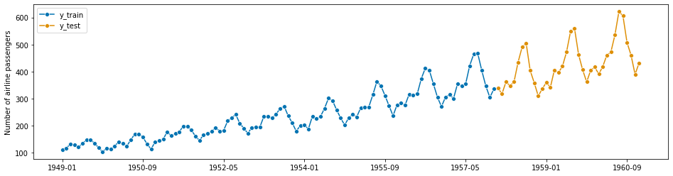
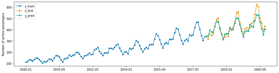
Example: In the example, we will us the same airline data as in Section 1.2. But, instead of predicting the next 3 years, we hold out the last 3 years of the airline data (below: y_test), and see how the forecaster would have performed three years ago, when asked to forecast the most recent 3 years (below: y_pred), from the years before (below: y_train). “how” is measured by a quantitative performance metric (below: mean_absolute_percentage_error). This is then considered as
an indication of how well the forecaster would perform in the coming 3 years (what was done in Section 1.2). This may or may not be a stretch depending on statistical assumptions and data properties (caution: it often is a stretch - past performance is in general not indicative of future performance).
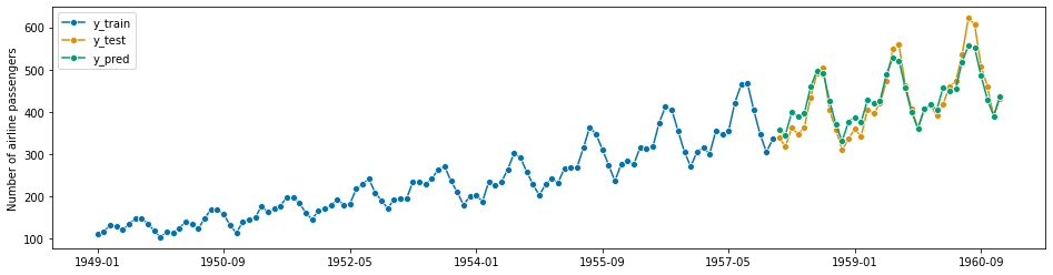
Step 1 - Splitting a historical data set in to a temporal train and test batch#
[38]:
from sktime.split import temporal_train_test_split
[39]:
y = load_airline()
y_train, y_test = temporal_train_test_split(y, test_size=36)
# we will try to forecast y_test from y_train
[40]:
# plotting for illustration
plot_series(y_train, y_test, labels=["y_train", "y_test"])
print(y_train.shape[0], y_test.shape[0])
Step 2 - Making forecasts for y_test from y_train#
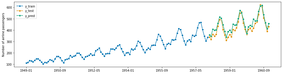
This is almost verbatim the workflow in Section 1.2, using y_train to predict the indices of y_test.
[41]:
# we can simply take the indices from `y_test` where they already are stored
fh = ForecastingHorizon(y_test.index, is_relative=False)

forecaster = NaiveForecaster(strategy="last", sp=12)

forecaster.fit(y_train)

# y_pred will contain the predictions
y_pred = forecaster.predict(fh)
[42]:
# plotting for illustration
plot_series(y_train, y_test, y_pred, labels=["y_train", "y_test", "y_pred"])
[42]:
(<Figure size 1152x288 with 1 Axes>,
 <AxesSubplot:ylabel='Number of airline passengers'>)

Steps 3 and 4 - Specifying a forecasting metric, evaluating on the test set#
The next step is to specify a forecasting metric. These are functions that return a number when input with prediction and actual series. They are different from sklearn metrics in that they accept series with indices rather than np.arrays. Forecasting metrics can be invoked in two ways:
using the lean function interface, e.g.,
mean_absolute_percentage_errorwhich is a python function(y_true : pd.Series, y_pred : pd.Series) -> floatusing the composable class interface, e.g.,
MeanAbsolutePercentageError, which is a python class, callable with the same signature
Casual users may opt to use the function interface. The class interface supports advanced use cases, such as parameter modification, custom metric composition, tuning over metric parameters (not covered in this tutorial)
[43]:
from sktime.performance_metrics.forecasting import mean_absolute_percentage_error
[44]:
# option 1: using the lean function interface
mean_absolute_percentage_error(y_test, y_pred, symmetric=False)
# note: the FIRST argument is the ground truth, the SECOND argument are the forecasts
#       the order matters for most metrics in general
[44]:
0.13189432350948402
To properly interpret numbers like this, it is useful to understand properties of the metric in question (e.g., lower is better), and to compare against suitable baselines and contender algorithms (see step 5).
[45]:
from sktime.performance_metrics.forecasting import MeanAbsolutePercentageError
[46]:
# option 2: using the composable class interface
mape = MeanAbsolutePercentageError(symmetric=False)
# the class interface allows to easily construct variants of the MAPE
#  e.g., the non-symmetric version
# it also allows for inspection of metric properties
#  e.g., are higher values better (answer: no)?
mape.get_tag("lower_is_better")
[46]:
True
[47]:
# evaluation works exactly like in option 2, but with the instantiated object
mape(y_test, y_pred)
[47]:
0.13189432350948402
NOTE: Some metrics, such as mean_absolute_scaled_error, also require the training set for evaluation. In this case, the training set should be passed as a y_train argument. Refer to the API reference on individual metrics.
NOTE: The workflow is the same for forecasters that make use of exogeneous data - no X is passed to the metrics.
Step 5 - Testing performance against benchmarks#
In general, forecast performances should be quantitatively tested against benchmark performances.
Currently (sktime v0.12.x), this is a roadmap development item. Contributions are very welcome.
1.3.1 The basic batch forecast evaluation workflow in a nutshell - function metric interface#
For convenience, we present the basic batch forecast evaluation workflow in one cell. This cell is using the lean function metric interface.
[48]:
from sktime.datasets import load_airline
from sktime.forecasting.base import ForecastingHorizon
from sktime.forecasting.naive import NaiveForecaster
from sktime.performance_metrics.forecasting import mean_absolute_percentage_error
from sktime.split import temporal_train_test_split
[49]:
# step 1: splitting historical data
y = load_airline()
y_train, y_test = temporal_train_test_split(y, test_size=36)

# step 2: running the basic forecasting workflow
fh = ForecastingHorizon(y_test.index, is_relative=False)
forecaster = NaiveForecaster(strategy="last", sp=12)
forecaster.fit(y_train)
y_pred = forecaster.predict(fh)

# step 3: specifying the evaluation metric and
# step 4: computing the forecast performance
mean_absolute_percentage_error(y_test, y_pred, symmetric=False)

# step 5: testing forecast performance against baseline
# under development
[49]:
0.13189432350948402
1.3.2 The basic batch forecast evaluation workflow in a nutshell - metric class interface#
For convenience, we present the basic batch forecast evaluation workflow in one cell. This cell is using the advanced class specification interface for metrics.
[50]:
from sktime.datasets import load_airline
from sktime.forecasting.base import ForecastingHorizon
from sktime.forecasting.naive import NaiveForecaster
from sktime.performance_metrics.forecasting import MeanAbsolutePercentageError
from sktime.split import temporal_train_test_split
[51]:
# step 1: splitting historical data
y = load_airline()
y_train, y_test = temporal_train_test_split(y, test_size=36)

# step 2: running the basic forecasting workflow
fh = ForecastingHorizon(y_test.index, is_relative=False)
forecaster = NaiveForecaster(strategy="last", sp=12)
forecaster.fit(y_train)
y_pred = forecaster.predict(fh)

# step 3: specifying the evaluation metric
mape = MeanAbsolutePercentageError(symmetric=False)
# if function interface is used, just use the function directly in step 4

# step 4: computing the forecast performance
mape(y_test, y_pred)

# step 5: testing forecast performance against baseline
# under development
[51]:
0.13189432350948402
A common use case requires the forecaster to regularly update with new data and make forecasts on a rolling basis. This is especially useful if the same kind of forecast has to be made at regular time points, e.g., daily or weekly. sktime forecasters support this type of deployment workflow via the update and update_predict methods.
The update method can be called when a forecaster is already fitted, to ingest new data and make updated forecasts - this is referred to as an “update step”.
After the update, the forecaster’s internal “now” state (the cutoff) is set to the latest time stamp seen in the update batch (assumed to be later than previously seen data).
The general pattern is as follows:
Specify a forecasting strategy
Specify a relative forecasting horizon
Fit the forecaster to an initial batch of data using
fitMake forecasts for the relative forecasting horizon, using
predictObtain new data; use
updateto ingest new dataMake forecasts using
predictfor the updated dataRepeat 5 and 6 as often as required
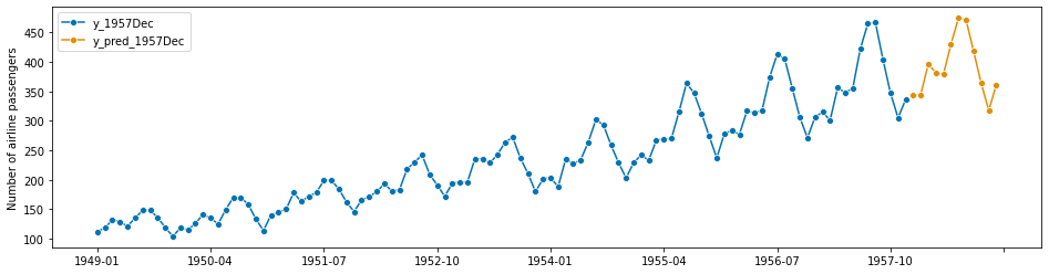
Example: suppose that, in the airline example, we want to make forecasts a year ahead, but every month, starting December 1957. The first few months, forecasts would be made as follows:
[52]:
from sktime.datasets import load_airline
from sktime.forecasting.ets import AutoETS
from sktime.utils.plotting import plot_series
[53]:
# we prepare the full data set for convenience
# note that in the scenario we will "know" only part of this at certain time points
y = load_airline()
[54]:
# December 1957
# this is the data known in December 1957
y_1957Dec = y[:-36]
# step 1: specifying the forecasting strategy
forecaster = AutoETS(auto=True, sp=12, n_jobs=-1)
# step 2: specifying the forecasting horizon: one year ahead, all months
fh = np.arange(1, 13)
# step 3: this is the first time we use the model, so we fit it
forecaster.fit(y_1957Dec)
# step 4: obtaining the first batch of forecasts for Jan 1958 - Dec 1958
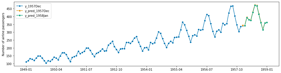
y_pred_1957Dec = forecaster.predict(fh)
[55]:
# plotting predictions and past data
plot_series(y_1957Dec, y_pred_1957Dec, labels=["y_1957Dec", "y_pred_1957Dec"])
[55]:
(<Figure size 1152x288 with 1 Axes>,
 <AxesSubplot:ylabel='Number of airline passengers'>)
[56]:
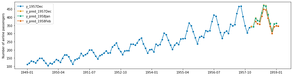
# January 1958

# new data is observed:
y_1958Jan = y[[-36]]

# step 5: we update the forecaster with the new data
forecaster.update(y_1958Jan)

# step 6: making forecasts with the updated data
y_pred_1958Jan = forecaster.predict(fh)
[57]:
# note that the fh is relative, so forecasts are automatically for 1 month later
#  i.e., from Feb 1958 to Jan 1959
y_pred_1958Jan
[57]:
1958-02    341.514630
1958-03    392.849241
1958-04    378.518543
1958-05    375.658188
1958-06    426.006944
1958-07    470.569699
1958-08    467.100443
1958-09    414.450926
1958-10    360.957054
1958-11    315.202860
1958-12    357.898458
1959-01    363.036833
Freq: M, dtype: float64
[58]:
# plotting predictions and past data
plot_series(
    y[:-35],
    y_pred_1957Dec,
    y_pred_1958Jan,
    labels=["y_1957Dec", "y_pred_1957Dec", "y_pred_1958Jan"],
)
[58]:
(<Figure size 1152x288 with 1 Axes>,
 <AxesSubplot:ylabel='Number of airline passengers'>)
[59]:
# February 1958

# new data is observed:
y_1958Feb = y[[-35]]

# step 5: we update the forecaster with the new data
forecaster.update(y_1958Feb)

# step 6: making forecasts with the updated data
y_pred_1958Feb = forecaster.predict(fh)
[60]:
# plotting predictions and past data
plot_series(
    y[:-35],
    y_pred_1957Dec,
    y_pred_1958Jan,
    y_pred_1958Feb,
    labels=["y_1957Dec", "y_pred_1957Dec", "y_pred_1958Jan", "y_pred_1958Feb"],
)
[60]:
(<Figure size 1152x288 with 1 Axes>,
 <AxesSubplot:ylabel='Number of airline passengers'>)
… and so on.
A shorthand for running first update and then predict is update_predict_single - for some algorithms, this may be more efficient than the separate calls to update and predict:
[61]:
# March 1958

# new data is observed:
y_1958Mar = y[[-34]]

# step 5&6: update/predict in one step
forecaster.update_predict_single(y_1958Mar, fh=fh)
[61]:
1958-04    349.161935
1958-05    346.920065
1958-06    394.051656
1958-07    435.839910
1958-08    433.316755
1958-09    384.841740
1958-10    335.535138
1958-11    293.171527
1958-12    333.275492
1959-01    338.595127
1959-02    336.983070
1959-03    388.121198
Freq: M, dtype: float64
In the rolling deployment mode, may be useful to move the estimator’s “now” state (the cutoff) to later, for example if no new data was observed, but time has progressed; or, if computations take too long, and forecasts have to be queried.
The update interface provides an option for this, via the update_params argument of update and other update functions.
If update_params is set to False, no model update computations are performed; only data is stored, and the internal “now” state (the cutoff) is set to the most recent date.
[62]:
# April 1958

# new data is observed:
y_1958Apr = y[[-33]]

# step 5: perform an update without re-computing the model parameters
forecaster.update(y_1958Apr, update_params=False)
[62]:
AutoETS(auto=True, n_jobs=-1, sp=12)
sktime can also simulate the update/predict deployment mode with a full batch of data.
This is not useful in deployment, as it requires all data to be available in advance; however, it is useful in playback, such as for simulations or model evaluation.
The update/predict playback mode can be called using update_predict and a re-sampling constructor which encodes the precise walk-forward scheme.
[63]:
# from sktime.datasets import load_airline
# from sktime.forecasting.ets import AutoETS
# from sktime.split import ExpandingWindowSplitter
# from sktime.utils.plotting import plot_series
NOTE: commented out - this part of the interface is currently undergoing a re-work. Contributions and PR are appreciated.
[64]:
# for playback, the full data needs to be loaded in advance
# y = load_airline()
[65]:
# step 1: specifying the forecasting strategy
# forecaster = AutoETS(auto=True, sp=12, n_jobs=-1)

# step 2: specifying the forecasting horizon
# fh - np.arange(1, 13)

# step 3: specifying the cross-validation scheme
# cv = ExpandingWindowSplitter()

# step 4: fitting the forecaster - fh should be passed here
# forecaster.fit(y[:-36], fh=fh)

# step 5: rollback
# y_preds = forecaster.update_predict(y, cv)
To evaluate forecasters with respect to their performance in rolling forecasting, the forecaster needs to be tested in a set-up mimicking rolling forecasting, usually on past data. Note that the batch back-testing as in Section 1.3 would not be an appropriate evaluation set-up for rolling deployment, as that tests only a single forecast batch.
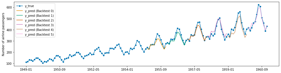
The advanced evaluation workflow can be carried out using the evaluate benchmarking function. evaluate takes as arguments: - a forecaster to be evaluated - a scikit-learn re-sampling strategy for temporal splitting (cv below), e.g., ExpandingWindowSplitter or SlidingWindowSplitter - a strategy (string): whether the forecaster should be always be refitted or just fitted once and then updated
[66]:
from sktime.forecasting.arima import AutoARIMA
from sktime.forecasting.model_evaluation import evaluate
from sktime.split import ExpandingWindowSplitter
[67]:
forecaster = AutoARIMA(sp=12, suppress_warnings=True)

cv = ExpandingWindowSplitter(
    step_length=12, fh=[1, 2, 3, 4, 5, 6, 7, 8, 9, 10, 11, 12], initial_window=72
)

df = evaluate(forecaster=forecaster, y=y, cv=cv, strategy="refit", return_data=True)

df.iloc[:, :5]
[67]:
| test_MeanAbsolutePercentageError | fit_time | pred_time | len_train_window | cutoff | |
|---|---|---|---|---|---|
| 0 | 0.061710 | 4.026436 | 0.006171 | 72 | 1954-12 |
| 1 | 0.050042 | 5.211994 | 0.006386 | 84 | 1955-12 |
| 2 | 0.029802 | 8.024385 | 0.005885 | 96 | 1956-12 |
| 3 | 0.053773 | 4.231226 | 0.005654 | 108 | 1957-12 |
| 4 | 0.073820 | 5.250797 | 0.006525 | 120 | 1958-12 |
| 5 | 0.030976 | 11.651850 | 0.006294 | 132 | 1959-12 |
[68]:
# visualization of a forecaster evaluation
fig, ax = plot_series(
    y,
    df["y_pred"].iloc[0],
    df["y_pred"].iloc[1],
    df["y_pred"].iloc[2],
    df["y_pred"].iloc[3],
    df["y_pred"].iloc[4],
    df["y_pred"].iloc[5],
    markers=["o", "", "", "", "", "", ""],
    labels=["y_true"] + ["y_pred (Backtest " + str(x) + ")" for x in range(6)],
)
ax.legend();
Todo: performance metrics, averages, and testing - contributions to sktime and the tutorial are welcome.
2. Forecasters in sktime - lookup, properties, main families#
This section summarizes how to:
search for forecasters in sktime
properties of forecasters, corresponding search options and tags
commonly used types of forecasters in
sktime
Generally, all forecasters available in sktime can be listed with the all_estimators command.
This will list all forecasters in sktime, even those whose soft dependencies are not installed.
[69]:
from sktime.registry import all_estimators

all_estimators("forecaster", as_dataframe=True)
[69]:
| name | estimator | |
|---|---|---|
| 0 | ARIMA | <class 'sktime.forecasting.arima.ARIMA'> |
| 1 | AutoARIMA | <class 'sktime.forecasting.arima.AutoARIMA'> |
| 2 | AutoETS | <class 'sktime.forecasting.ets.AutoETS'> |
| 3 | AutoEnsembleForecaster | <class 'sktime.forecasting.compose._ensemble.A... |
| 4 | BATS | <class 'sktime.forecasting.bats.BATS'> |
| 5 | BaggingForecaster | <class 'sktime.forecasting.compose._bagging.Ba... |
| 6 | ColumnEnsembleForecaster | <class 'sktime.forecasting.compose._column_ens... |
| 7 | ConformalIntervals | <class 'sktime.forecasting.conformal.Conformal... |
| 8 | Croston | <class 'sktime.forecasting.croston.Croston'> |
| 9 | DirRecTabularRegressionForecaster | <class 'sktime.forecasting.compose._reduce.Dir... |
| 10 | DirRecTimeSeriesRegressionForecaster | <class 'sktime.forecasting.compose._reduce.Dir... |
| 11 | DirectTabularRegressionForecaster | <class 'sktime.forecasting.compose._reduce.Dir... |
| 12 | DirectTimeSeriesRegressionForecaster | <class 'sktime.forecasting.compose._reduce.Dir... |
| 13 | DontUpdate | <class 'sktime.forecasting.stream._update.Dont... |
| 14 | DynamicFactor | <class 'sktime.forecasting.dynamic_factor.Dyna... |
| 15 | EnsembleForecaster | <class 'sktime.forecasting.compose._ensemble.E... |
| 16 | ExponentialSmoothing | <class 'sktime.forecasting.exp_smoothing.Expon... |
| 17 | ForecastX | <class 'sktime.forecasting.compose._pipeline.F... |
| 18 | ForecastingGridSearchCV | <class 'sktime.forecasting.model_selection._tu... |
| 19 | ForecastingPipeline | <class 'sktime.forecasting.compose._pipeline.F... |
| 20 | ForecastingRandomizedSearchCV | <class 'sktime.forecasting.model_selection._tu... |
| 21 | MultioutputTabularRegressionForecaster | <class 'sktime.forecasting.compose._reduce.Mul... |
| 22 | MultioutputTimeSeriesRegressionForecaster | <class 'sktime.forecasting.compose._reduce.Mul... |
| 23 | MultiplexForecaster | <class 'sktime.forecasting.compose._multiplexe... |
| 24 | NaiveForecaster | <class 'sktime.forecasting.naive.NaiveForecast... |
| 25 | NaiveVariance | <class 'sktime.forecasting.naive.NaiveVariance'> |
| 26 | OnlineEnsembleForecaster | <class 'sktime.forecasting.online_learning._on... |
| 27 | PolynomialTrendForecaster | <class 'sktime.forecasting.trend.PolynomialTre... |
| 28 | Prophet | <class 'sktime.forecasting.fbprophet.Prophet'> |
| 29 | ReconcilerForecaster | <class 'sktime.forecasting.reconcile.Reconcile... |
| 30 | RecursiveTabularRegressionForecaster | <class 'sktime.forecasting.compose._reduce.Rec... |
| 31 | RecursiveTimeSeriesRegressionForecaster | <class 'sktime.forecasting.compose._reduce.Rec... |
| 32 | SARIMAX | <class 'sktime.forecasting.sarimax.SARIMAX'> |
| 33 | STLForecaster | <class 'sktime.forecasting.trend.STLForecaster'> |
| 34 | StackingForecaster | <class 'sktime.forecasting.compose._stack.Stac... |
| 35 | StatsForecastAutoARIMA | <class 'sktime.forecasting.statsforecast.Stats... |
| 36 | TBATS | <class 'sktime.forecasting.tbats.TBATS'> |
| 37 | ThetaForecaster | <class 'sktime.forecasting.theta.ThetaForecast... |
| 38 | TransformedTargetForecaster | <class 'sktime.forecasting.compose._pipeline.T... |
| 39 | TrendForecaster | <class 'sktime.forecasting.trend.TrendForecast... |
| 40 | UnobservedComponents | <class 'sktime.forecasting.structural.Unobserv... |
| 41 | UpdateEvery | <class 'sktime.forecasting.stream._update.Upda... |
| 42 | UpdateRefitsEvery | <class 'sktime.forecasting.stream._update.Upda... |
| 43 | VAR | <class 'sktime.forecasting.var.VAR'> |
| 44 | VARMAX | <class 'sktime.forecasting.varmax.VARMAX'> |
| 45 | VECM | <class 'sktime.forecasting.vecm.VECM'> |
The entries of the last column of the resulting dataframe are classes which could be directly used for construction, or simply inspected for the correct import path.
For logic that loops over forecasters, the default output format may be more convenient:
[70]:
forecaster_list = all_estimators("forecaster", as_dataframe=False)

# this returns a list of (name, estimator) tuples
forecaster_list[0]
[70]:
('ARIMA', sktime.forecasting.arima.ARIMA)
All forecasters sktime have so-called tags which describe properties of the estimator, e.g., whether it is multivariate, probabilistic, or not. Use of tags, inspection, and retrieval will be described in this section.
Every forecaster has tags, which are key-value pairs that can describe capabilities or internal implementation details.
The most important “capability” style tags are the following:
requires-fh-in-fit - a boolean. Whether the forecaster requires the forecasting horizon fh already in fit (True), or whether it can be passed late in predict (False).
scitype:y - a string. Whether the forecaster is univariate ("univariate"), strictly multivariate ("multivariate"), or can deal with any number of variables ("both").
capability:pred_int - a boolean. Whether the forecaster can return probabilistic predictions via predict_interval etc, see Section 1.5.
ignores-exogeneous-X - a boolean. Whether the forecaster makes use of exogeneous variables X (False) or not (True). If the forecaster does not use X, it can still be passed for interface uniformity, and will be ignored.
handles-missing-data - a boolean. Whether the forecaster can deal with missing data in the inputs X or y.
Tags of a forecaster instance can be inspected via the get_tags (lists all tags) and get_tag (gets value for one tag) methods.
Tag values may depend on hyper-parameter choices.
[71]:
from sktime.forecasting.arima import ARIMA

ARIMA().get_tags()
[71]:
{'scitype:y': 'univariate',
 'ignores-exogeneous-X': False,
 'capability:pred_int': True,
 'handles-missing-data': True,
 'y_inner_mtype': 'pd.Series',
 'X_inner_mtype': 'pd.DataFrame',
 'requires-fh-in-fit': False,
 'X-y-must-have-same-index': True,
 'enforce_index_type': None,
 'fit_is_empty': False,
 'python_version': None,
 'python_dependencies': 'pmdarima'}
The y_inner_mtype and X_inner_mtype indicate whether the forecaster can deal with panel or hierarchical data natively - if an panel or hierarchical mtype occurs here, it does (see data types tutorial).
An explanation for all tags can be obtained using the all_tags utility, see Section 2.2.3.
To list forecasters with their tags, the all_estimators utility can be used with its return_tags argument.
The resulting data frame can then be used for table queries or sub-setting.
[72]:
from sktime.registry import all_estimators

all_estimators(
    "forecaster", as_dataframe=True, return_tags=["scitype:y", "requires-fh-in-fit"]
)
[72]:
| name | estimator | scitype:y | requires-fh-in-fit | |
|---|---|---|---|---|
| 0 | ARIMA | <class 'sktime.forecasting.arima.ARIMA'> | univariate | False |
| 1 | AutoARIMA | <class 'sktime.forecasting.arima.AutoARIMA'> | univariate | False |
| 2 | AutoETS | <class 'sktime.forecasting.ets.AutoETS'> | univariate | False |
| 3 | AutoEnsembleForecaster | <class 'sktime.forecasting.compose._ensemble.A... | univariate | False |
| 4 | BATS | <class 'sktime.forecasting.bats.BATS'> | univariate | False |
| 5 | BaggingForecaster | <class 'sktime.forecasting.compose._bagging.Ba... | univariate | False |
| 6 | ColumnEnsembleForecaster | <class 'sktime.forecasting.compose._column_ens... | both | False |
| 7 | ConformalIntervals | <class 'sktime.forecasting.conformal.Conformal... | univariate | False |
| 8 | Croston | <class 'sktime.forecasting.croston.Croston'> | univariate | False |
| 9 | DirRecTabularRegressionForecaster | <class 'sktime.forecasting.compose._reduce.Dir... | univariate | True |
| 10 | DirRecTimeSeriesRegressionForecaster | <class 'sktime.forecasting.compose._reduce.Dir... | univariate | True |
| 11 | DirectTabularRegressionForecaster | <class 'sktime.forecasting.compose._reduce.Dir... | univariate | True |
| 12 | DirectTimeSeriesRegressionForecaster | <class 'sktime.forecasting.compose._reduce.Dir... | univariate | True |
| 13 | DontUpdate | <class 'sktime.forecasting.stream._update.Dont... | univariate | False |
| 14 | DynamicFactor | <class 'sktime.forecasting.dynamic_factor.Dyna... | multivariate | False |
| 15 | EnsembleForecaster | <class 'sktime.forecasting.compose._ensemble.E... | univariate | False |
| 16 | ExponentialSmoothing | <class 'sktime.forecasting.exp_smoothing.Expon... | univariate | False |
| 17 | ForecastX | <class 'sktime.forecasting.compose._pipeline.F... | univariate | True |
| 18 | ForecastingGridSearchCV | <class 'sktime.forecasting.model_selection._tu... | both | False |
| 19 | ForecastingPipeline | <class 'sktime.forecasting.compose._pipeline.F... | both | False |
| 20 | ForecastingRandomizedSearchCV | <class 'sktime.forecasting.model_selection._tu... | both | False |
| 21 | MultioutputTabularRegressionForecaster | <class 'sktime.forecasting.compose._reduce.Mul... | univariate | True |
| 22 | MultioutputTimeSeriesRegressionForecaster | <class 'sktime.forecasting.compose._reduce.Mul... | univariate | True |
| 23 | MultiplexForecaster | <class 'sktime.forecasting.compose._multiplexe... | both | False |
| 24 | NaiveForecaster | <class 'sktime.forecasting.naive.NaiveForecast... | univariate | False |
| 25 | NaiveVariance | <class 'sktime.forecasting.naive.NaiveVariance'> | univariate | False |
| 26 | OnlineEnsembleForecaster | <class 'sktime.forecasting.online_learning._on... | univariate | False |
| 27 | PolynomialTrendForecaster | <class 'sktime.forecasting.trend.PolynomialTre... | univariate | False |
| 28 | Prophet | <class 'sktime.forecasting.fbprophet.Prophet'> | univariate | False |
| 29 | ReconcilerForecaster | <class 'sktime.forecasting.reconcile.Reconcile... | univariate | False |
| 30 | RecursiveTabularRegressionForecaster | <class 'sktime.forecasting.compose._reduce.Rec... | univariate | False |
| 31 | RecursiveTimeSeriesRegressionForecaster | <class 'sktime.forecasting.compose._reduce.Rec... | univariate | False |
| 32 | SARIMAX | <class 'sktime.forecasting.sarimax.SARIMAX'> | univariate | False |
| 33 | STLForecaster | <class 'sktime.forecasting.trend.STLForecaster'> | univariate | False |
| 34 | StackingForecaster | <class 'sktime.forecasting.compose._stack.Stac... | univariate | True |
| 35 | StatsForecastAutoARIMA | <class 'sktime.forecasting.statsforecast.Stats... | univariate | False |
| 36 | TBATS | <class 'sktime.forecasting.tbats.TBATS'> | univariate | False |
| 37 | ThetaForecaster | <class 'sktime.forecasting.theta.ThetaForecast... | univariate | False |
| 38 | TransformedTargetForecaster | <class 'sktime.forecasting.compose._pipeline.T... | both | False |
| 39 | TrendForecaster | <class 'sktime.forecasting.trend.TrendForecast... | univariate | False |
| 40 | UnobservedComponents | <class 'sktime.forecasting.structural.Unobserv... | univariate | False |
| 41 | UpdateEvery | <class 'sktime.forecasting.stream._update.Upda... | univariate | False |
| 42 | UpdateRefitsEvery | <class 'sktime.forecasting.stream._update.Upda... | univariate | False |
| 43 | VAR | <class 'sktime.forecasting.var.VAR'> | multivariate | False |
| 44 | VARMAX | <class 'sktime.forecasting.varmax.VARMAX'> | multivariate | False |
| 45 | VECM | <class 'sktime.forecasting.vecm.VECM'> | multivariate | False |
To filter beforehand on certain tags and tag values, the filter_tags argument can be used:
[73]:
# this lists all forecasters that can deal with multivariate data
all_estimators(
    "forecaster", as_dataframe=True, filter_tags={"scitype:y": ["multivariate", "both"]}
)
[73]:
| name | estimator | |
|---|---|---|
| 0 | ColumnEnsembleForecaster | <class 'sktime.forecasting.compose._column_ens... |
| 1 | DynamicFactor | <class 'sktime.forecasting.dynamic_factor.Dyna... |
| 2 | ForecastingGridSearchCV | <class 'sktime.forecasting.model_selection._tu... |
| 3 | ForecastingPipeline | <class 'sktime.forecasting.compose._pipeline.F... |
| 4 | ForecastingRandomizedSearchCV | <class 'sktime.forecasting.model_selection._tu... |
| 5 | MultiplexForecaster | <class 'sktime.forecasting.compose._multiplexe... |
| 6 | TransformedTargetForecaster | <class 'sktime.forecasting.compose._pipeline.T... |
| 7 | VAR | <class 'sktime.forecasting.var.VAR'> |
| 8 | VARMAX | <class 'sktime.forecasting.varmax.VARMAX'> |
| 9 | VECM | <class 'sktime.forecasting.vecm.VECM'> |
Important note: as said above, tag values can depend on hyper-parameter settings, e.g., a ForecastingPipeline can handle multivariate data only if the forecaster in it can handle multivariate data.
In retrieval as above, the tags for a class are usually set to indicate the most general potential value, e.g., if for some parameter choice the estimator can handle multivariate, it will appear on the list.
To list all forecaster tags with an explanation of the tag, the all_tags utility can be used:
[74]:
import pandas as pd

from sktime.registry import all_tags

# wrapping this in a pandas DataFrame for pretty display
pd.DataFrame(all_tags(estimator_types="forecaster"))[[0, 3]]
[74]:
| 0 | 3 | |
|---|---|---|
| 0 | X-y-must-have-same-index | do X/y in fit/update and X/fh in predict have ... |
| 1 | X_inner_mtype | which machine type(s) is the internal _fit/_pr... |
| 2 | capability:pred_int | does the forecaster implement predict_interval... |
| 3 | capability:pred_var | does the forecaster implement predict_variance? |
| 4 | enforce_index_type | passed to input checks, input conversion index... |
| 5 | ignores-exogeneous-X | does forecaster ignore exogeneous data (X)? |
| 6 | requires-fh-in-fit | does forecaster require fh passed already in f... |
| 7 | scitype:y | which series type does the forecaster support?... |
| 8 | y_inner_mtype | which machine type(s) is the internal _fit/_pr... |
sktime supports a number of commonly used forecasters, many of them interfaced from state-of-art forecasting packages. All forecasters are available under the unified sktime interface.
Some classes that are currently stably supported are:
ExponentialSmoothing,ThetaForecaster, andautoETSfromstatsmodelsARIMAandAutoARIMAfrompmdarimaAutoARIMAfromstatsforecastBATSandTBATSfromtbatsPolynomialTrendfor forecasting polynomial trendsProphetwhich interfaces Facebookprophet
This is not the full list, use all_estimators as demonstrated in Sections 2.1 and 2.2 for that.
For illustration, all estimators below will be presented on the basic forecasting workflow - though they also support the advanced forecasting and evaluation workflows under the unified sktime interface (see Section 1).
For use in the other workflows, simply replace the “forecaster specification block” (”forecaster=”) by the forecaster specification block in the examples presented below.
[75]:
# imports necessary for this chapter
from sktime.datasets import load_airline
from sktime.forecasting.base import ForecastingHorizon
from sktime.performance_metrics.forecasting import mean_absolute_percentage_error
from sktime.split import temporal_train_test_split
from sktime.utils.plotting import plot_series

# data loading for illustration (see section 1 for explanation)
y = load_airline()
y_train, y_test = temporal_train_test_split(y, test_size=36)
fh = ForecastingHorizon(y_test.index, is_relative=False)
sktime interfaces a number of statistical forecasting algorithms from statsmodels: exponential smoothing, theta, and auto-ETS.
For example, to use exponential smoothing with an additive trend component and multiplicative seasonality on the airline data set, we can write the following. Note that since this is monthly data, a good choic for seasonal periodicity (sp) is 12 (= hypothesized periodicity of a year).
[76]:
from sktime.forecasting.exp_smoothing import ExponentialSmoothing
[77]:
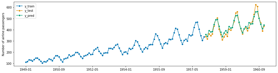
forecaster = ExponentialSmoothing(trend="add", seasonal="additive", sp=12)

forecaster.fit(y_train)
y_pred = forecaster.predict(fh)
plot_series(y_train, y_test, y_pred, labels=["y_train", "y_test", "y_pred"])
mean_absolute_percentage_error(y_test, y_pred, symmetric=False)
[77]:
0.05114163237371178
The exponential smoothing of state space model can also be automated similar to the ets function in R. This is implemented in the AutoETS forecaster.
[78]:
from sktime.forecasting.ets import AutoETS
[79]:
forecaster = AutoETS(auto=True, sp=12, n_jobs=-1)

forecaster.fit(y_train)
y_pred = forecaster.predict(fh)
plot_series(y_train, y_test, y_pred, labels=["y_train", "y_test", "y_pred"])
mean_absolute_percentage_error(y_test, y_pred, symmetric=False)
[79]:
0.06186318537056982
[80]:
# todo: explain Theta; explain how to get theta-lines
sktime interfaces pmdarima for its ARIMA class models. For a classical ARIMA model with set parameters, use the ARIMA forecaster:
[81]:
from sktime.forecasting.arima import ARIMA
[82]:
forecaster = ARIMA(
    order=(1, 1, 0), seasonal_order=(0, 1, 0, 12), suppress_warnings=True
)

forecaster.fit(y_train)
y_pred = forecaster.predict(fh)
plot_series(y_train, y_test, y_pred, labels=["y_train", "y_test", "y_pred"])
mean_absolute_percentage_error(y_test, y_pred, symmetric=False)
[82]:
0.04356744885278522

AutoARIMA is an automatically tuned ARIMA variant that obtains the optimal pdq parameters automatically:
[83]:
from sktime.forecasting.arima import AutoARIMA
[84]:
forecaster = AutoARIMA(sp=12, suppress_warnings=True)

forecaster.fit(y_train)
y_pred = forecaster.predict(fh)
plot_series(y_train, y_test, y_pred, labels=["y_train", "y_test", "y_pred"])
mean_absolute_percentage_error(y_test, y_pred, symmetric=False)
[84]:
0.041489714388809135

[85]:
forecaster = AutoARIMA(sp=12, suppress_warnings=True)

forecaster.fit(y_train)
y_pred = forecaster.predict(fh)
plot_series(y_train, y_test, y_pred, labels=["y_train", "y_test", "y_pred"])
mean_absolute_percentage_error(y_pred, y_test)
[85]:
0.040936759322166255

[86]:
# to obtain the fitted parameters, run
forecaster.get_fitted_params()
# should these not include pdq?
[86]:
{'ar.L1': -0.24111779230017605,
 'sigma2': 92.74986650446229,
 'order': (1, 1, 0),
 'seasonal_order': (0, 1, 0, 12),
 'aic': 704.0011679023331,
 'aicc': 704.1316026849419,
 'bic': 709.1089216855343,
 'hqic': 706.0650836393346}
sktime interfaces BATS and TBATS from the `tbats <intive-DataScience/tbats>`__ package.
[87]:
from sktime.forecasting.bats import BATS
[88]:
forecaster = BATS(sp=12, use_trend=True, use_box_cox=False)

forecaster.fit(y_train)
y_pred = forecaster.predict(fh)
plot_series(y_train, y_test, y_pred, labels=["y_train", "y_test", "y_pred"])
mean_absolute_percentage_error(y_test, y_pred, symmetric=False)
[88]:
0.08185558959286515

[89]:
from sktime.forecasting.tbats import TBATS
[90]:
forecaster = TBATS(sp=12, use_trend=True, use_box_cox=False)

forecaster.fit(y_train)
y_pred = forecaster.predict(fh)
plot_series(y_train, y_test, y_pred, labels=["y_train", "y_test", "y_pred"])
mean_absolute_percentage_error(y_test, y_pred, symmetric=False)
[90]:
0.08024090844021753

sktime provides an interface to `fbprophet <facebook/prophet>`__ by Facebook.
[91]:
from sktime.forecasting.fbprophet import Prophet
The current interface does not support period indices, only pd.DatetimeIndex. Consider improving this by contributing the sktime.
[92]:
# Convert index to pd.DatetimeIndex
z = y.copy()
z = z.to_timestamp(freq="M")
z_train, z_test = temporal_train_test_split(z, test_size=36)
[93]:
forecaster = Prophet(
    seasonality_mode="multiplicative",
    n_changepoints=int(len(y_train) / 12),
    add_country_holidays={"country_name": "Germany"},
    yearly_seasonality=True,
    weekly_seasonality=False,
    daily_seasonality=False,
)

forecaster.fit(z_train)
y_pred = forecaster.predict(fh.to_relative(cutoff=y_train.index[-1]))
y_pred.index = y_test.index

plot_series(y_train, y_test, y_pred, labels=["y_train", "y_test", "y_pred"])
mean_absolute_percentage_error(y_test, y_pred, symmetric=False)
[93]:
0.07276862950407971
We can also use the `UnobservedComponents <https://www.statsmodels.org/stable/generated/statsmodels.tsa.statespace.structural.UnobservedComponents.html>`__ class from `statsmodels <https://www.statsmodels.org/stable/index.html>`__ to generate predictions using a state space model.
[94]:
from sktime.forecasting.structural import UnobservedComponents
[95]:
# We can model seasonality using Fourier modes as in the Prophet model.
forecaster = UnobservedComponents(
    level="local linear trend", freq_seasonal=[{"period": 12, "harmonics": 10}]
)

forecaster.fit(y_train)
y_pred = forecaster.predict(fh)
plot_series(y_train, y_test, y_pred, labels=["y_train", "y_test", "y_pred"])
mean_absolute_percentage_error(y_test, y_pred, symmetric=False)
[95]:
0.0497366365924174
sktime interfaces StatsForecast for its AutoARIMA class models. AutoARIMA is an automatically tuned ARIMA variant that obtains the optimal pdq parameters automatically:
[96]:
from sktime.forecasting.statsforecast import StatsForecastAutoARIMA
[97]:
forecaster = StatsForecastAutoARIMA(sp=12)

forecaster.fit(y_train)
y_pred = forecaster.predict(fh)
plot_series(y_train, y_test, y_pred, labels=["y_train", "y_test", "y_pred"])
mean_absolute_percentage_error(y_pred, y_test)
[97]:
0.04093539044441262

3. Advanced composition patterns - pipelines, reduction, autoML, and more#
sktime supports a number of advanced composition patterns to create forecasters out of simpler components:
Reduction - building a forecaster from estimators of “simpler” scientific types, like
scikit-learnregressors. A common example is feature/label tabulation by rolling window, aka the “direct reduction strategy”.Tuning - determining values for hyper-parameters of a forecaster in a data-driven manner. A common example is grid search on temporally rolling re-sampling of train/test splits.
Pipelining - concatenating transformers with a forecaster to obtain one forecaster. A common example is detrending and deseasonalizing then forecasting, an instance of this is the common “STL forecaster”.
AutoML, also known as automated model selection - using automated tuning strategies to select not only hyper-parameters but entire forecasting strategies. A common example is on-line multiplexer tuning.
For illustration, all estimators below will be presented on the basic forecasting workflow - though they also support the advanced forecasting and evaluation workflows under the unified sktime interface (see Section 1).
For use in the other workflows, simply replace the “forecaster specification block” (”forecaster=”) by the forecaster specification block in the examples presented below.
[98]:
# imports necessary for this chapter
from sktime.datasets import load_airline
from sktime.forecasting.base import ForecastingHorizon
from sktime.performance_metrics.forecasting import mean_absolute_percentage_error
from sktime.split import temporal_train_test_split
from sktime.utils.plotting import plot_series

# data loading for illustration (see section 1 for explanation)
y = load_airline()
y_train, y_test = temporal_train_test_split(y, test_size=36)
fh = ForecastingHorizon(y_test.index, is_relative=False)
sktime provides a meta-estimator that allows the use of any scikit-learn estimator for forecasting.
modular and compatible with scikit-learn, so that we can easily apply any scikit-learn regressor to solve our forecasting problem,
parametric and tuneable, allowing us to tune hyper-parameters such as the window length or strategy to generate forecasts
adaptive, in the sense that it adapts the scikit-learn’s estimator interface to that of a forecaster, making sure that we can tune and properly evaluate our model
Example: we will define a tabulation reduction strategy to convert a k-nearest neighbors regressor (sklearn KNeighborsRegressor) into a forecaster. The composite algorithm is an object compliant with the sktime forecaster interface (picture: big robot), and contains the regressor as a parameter accessible component (picture: little robot). In fit, the composite algorithm uses a sliding window strategy to tabulate the data, and fit the regressor to the tabulated data (picture:
left half). In predict, the composite algorithm presents the regressor with the last observed window to obtain predictions (picture: right half).
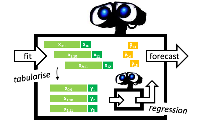
Below, the composite is constructed using the shorthand function make_reduction which produces a sktime estimator of forecaster scitype. It is called with a constructed scikit-learn regressor, regressor, and additional parameter which can be later tuned as hyper-parameters
[99]:
from sklearn.neighbors import KNeighborsRegressor

from sktime.forecasting.compose import make_reduction
[100]:
regressor = KNeighborsRegressor(n_neighbors=1)
forecaster = make_reduction(regressor, window_length=15, strategy="recursive")
[101]:
forecaster.fit(y_train)
y_pred = forecaster.predict(fh)
plot_series(y_train, y_test, y_pred, labels=["y_train", "y_test", "y_pred"])
mean_absolute_percentage_error(y_test, y_pred, symmetric=False)
[101]:
0.12887507224382988

In the above example we use the “recursive” reduction strategy. Other implemented strategies are: * “direct”, * “dirrec”, * “multioutput”.
Parameters can be inspected using scikit-learn compatible get_params functionality (and set using set_params). This provides tunable and nested access to parameters of the KNeighborsRegressor (as estimator_etc), and the window_length of the reduction strategy. Note that the strategy is not accessible, as underneath the utility function this is mapped on separate algorithm classes. For tuning over algorithms, see the “autoML” section below.
[102]:
forecaster.get_params()
[102]:
{'estimator__algorithm': 'auto',
 'estimator__leaf_size': 30,
 'estimator__metric': 'minkowski',
 'estimator__metric_params': None,
 'estimator__n_jobs': None,
 'estimator__n_neighbors': 1,
 'estimator__p': 2,
 'estimator__weights': 'uniform',
 'estimator': KNeighborsRegressor(n_neighbors=1),
 'transformers': None,
 'window_length': 15}
A common composition motif is pipelining: for example, first deseasonalizing or detrending the data, then forecasting the detrended/deseasonalized series. When forecasting, one needs to add the trend and seasonal component back to the data.
3.2.1 The basic forecasting pipeline#
sktime provides a generic pipeline object for this kind of composite modelling, the TransformedTargetForecaster. It chains an arbitrary number of transformations with a forecaster. The transformations can either be pre-processing transformations or a post-processing transformations. An example of a forecaster with pre-processing transformations can be seen below.
[103]:
from sktime.forecasting.arima import ARIMA
from sktime.forecasting.compose import TransformedTargetForecaster
from sktime.transformations.series.detrend import Deseasonalizer
[104]:
forecaster = TransformedTargetForecaster(
    [
        ("deseasonalize", Deseasonalizer(model="multiplicative", sp=12)),
        ("forecast", ARIMA()),
    ]
)

forecaster.fit(y_train)
y_pred = forecaster.predict(fh)
plot_series(y_train, y_test, y_pred, labels=["y_train", "y_test", "y_pred"])
mean_absolute_percentage_error(y_test, y_pred, symmetric=False)
[104]:
0.13969973496344534

In the above example, the TransformedTargetForecaster is constructed with a list of steps, each a pair of name and estimator, where the last estimator is a forecaster scitype. The pre-processing transformers should be series-to-series transformers which possess both a transform and an inverse_transform method. The resulting estimator is of forecaster scitype and has all interface defining methods. In fit, all transformers apply fit_transforms to the data, then the
forecaster’s fit; in predict, first the forecaster’s predict is applied, then the transformers’ inverse_transform in reverse order.
The same pipeline, as above, can also be constructed with the multiplication dunder method *.
This creates a TransformedTargetForecaster as above, with components given default names.
[105]:
forecaster = Deseasonalizer(model="multiplicative", sp=12) * ARIMA()
forecaster
[105]:
TransformedTargetForecaster(steps=[Deseasonalizer(model='multiplicative',
                                                  sp=12),
                                   ARIMA()])
The names in a dunder constructed pipeline are made unique in case, e.g., two deseasonalizers are used.
Example of a multiple seasonality model:
[106]:
forecaster = (
    Deseasonalizer(model="multiplicative", sp=12)
    * Deseasonalizer(model="multiplicative", sp=3)
    * ARIMA()
)

forecaster.get_params()
[106]:
{'steps': [Deseasonalizer(model='multiplicative', sp=12),
  Deseasonalizer(model='multiplicative', sp=3),
  ARIMA()],
 'Deseasonalizer_1': Deseasonalizer(model='multiplicative', sp=12),
 'Deseasonalizer_2': Deseasonalizer(model='multiplicative', sp=3),
 'ARIMA': ARIMA(),
 'Deseasonalizer_1__model': 'multiplicative',
 'Deseasonalizer_1__sp': 12,
 'Deseasonalizer_2__model': 'multiplicative',
 'Deseasonalizer_2__sp': 3,
 'ARIMA__concentrate_scale': False,
 'ARIMA__enforce_invertibility': True,
 'ARIMA__enforce_stationarity': True,
 'ARIMA__hamilton_representation': False,
 'ARIMA__maxiter': 50,
 'ARIMA__measurement_error': False,
 'ARIMA__method': 'lbfgs',
 'ARIMA__mle_regression': True,
 'ARIMA__order': (1, 0, 0),
 'ARIMA__out_of_sample_size': 0,
 'ARIMA__scoring': 'mse',
 'ARIMA__scoring_args': None,
 'ARIMA__seasonal_order': (0, 0, 0, 0),
 'ARIMA__simple_differencing': False,
 'ARIMA__start_params': None,
 'ARIMA__suppress_warnings': False,
 'ARIMA__time_varying_regression': False,
 'ARIMA__trend': None,
 'ARIMA__with_intercept': True}
We can also create a pipeline with post-processing transformations, these are transformations after the forecaster, in a dunder pipeline or a TransformedTargetForecaster.
Below is an example of a multiple seasonality model, with integer rounding post-processing of the predictions:
[107]:
from sktime.transformations.series.func_transform import FunctionTransformer

forecaster = ARIMA() * FunctionTransformer(lambda y: y.round())
forecaster.fit_predict(y, fh=fh).head(3)
[107]:
1958-01    334.0
1958-02    338.0
1958-03    317.0
Freq: M, dtype: float64
Both pre- and post-processing transformers can be present, in this case the post-processing transformations will be applied after the inverse-transform of the pre-processing ones.
[108]:
forecaster = (
    Deseasonalizer(model="multiplicative", sp=12)
    * Deseasonalizer(model="multiplicative", sp=3)
    * ARIMA()
    * FunctionTransformer(lambda y: y.round())
)

forecaster.fit_predict(y_train, fh=fh).head(3)
[108]:
1958-01    339.0
1958-02    334.0
1958-03    381.0
Freq: M, dtype: float64
3.2.2 The Detrender as pipeline component#
For detrending, we can use the Detrender. This is an estimator of series-to-transformer scitype that wraps an arbitrary forecaster. For example, for linear detrending, we can use PolynomialTrendForecaster to fit a linear trend, and then subtract/add it using the Detrender transformer inside TransformedTargetForecaster.
To understand better what happens, we first examine the detrender separately:
[109]:
from sktime.forecasting.trend import PolynomialTrendForecaster
from sktime.transformations.series.detrend import Detrender
[110]:
# linear detrending
forecaster = PolynomialTrendForecaster(degree=1)
transformer = Detrender(forecaster=forecaster)
yt = transformer.fit_transform(y_train)

# internally, the Detrender uses the in-sample predictions
# of the PolynomialTrendForecaster
forecaster = PolynomialTrendForecaster(degree=1)
fh_ins = -np.arange(len(y_train))  # in-sample forecasting horizon
y_pred = forecaster.fit(y_train).predict(fh=fh_ins)

plot_series(
    y_train, y_pred, yt, labels=["y_train", "fitted linear trend", "residuals"]
);
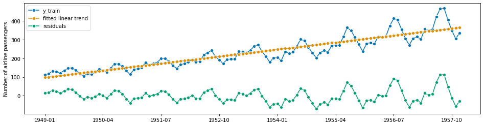
Since the Detrender is of scitype series-to-series-transformer, it can be used in the TransformedTargetForecaster for detrending any forecaster:
[111]:
forecaster = TransformedTargetForecaster(
    [
        ("deseasonalize", Deseasonalizer(model="multiplicative", sp=12)),
        ("detrend", Detrender(forecaster=PolynomialTrendForecaster(degree=1))),
        ("forecast", ARIMA()),
    ]
)

forecaster.fit(y_train)
y_pred = forecaster.predict(fh)
plot_series(y_train, y_test, y_pred, labels=["y_train", "y_test", "y_pred"])
mean_absolute_percentage_error(y_test, y_pred, symmetric=False)
[111]:
0.05610168219854761

3.2.3 Complex pipeline composites and parameter inspection#
sktime follows the scikit-learn philosophy of composability and nested parameter inspection. As long as an estimator has the right scitype, it can be used as part of any composition principle requiring that scitype. Above, we have already seen the example of a forecaster inside a Detrender, which is an estimator of scitype series-to-series-transformer, with one component of forecaster scitype. Similarly, in a TransformedTargetForecaster, we can use the reduction composite from
Section 3.1 as the last forecaster element in the pipeline, which inside has an estimator of tabular regressor scitype, the KNeighborsRegressor:
[112]:
from sklearn.neighbors import KNeighborsRegressor

from sktime.forecasting.compose import make_reduction
[113]:
forecaster = TransformedTargetForecaster(
    [
        ("deseasonalize", Deseasonalizer(model="multiplicative", sp=12)),
        ("detrend", Detrender(forecaster=PolynomialTrendForecaster(degree=1))),
        (
            "forecast",
            make_reduction(
                KNeighborsRegressor(),
                window_length=15,
                strategy="recursive",
            ),
        ),
    ]
)

forecaster.fit(y_train)
y_pred = forecaster.predict(fh)
plot_series(y_train, y_test, y_pred, labels=["y_train", "y_test", "y_pred"])
mean_absolute_percentage_error(y_test, y_pred, symmetric=False)
[113]:
0.058708387889316475
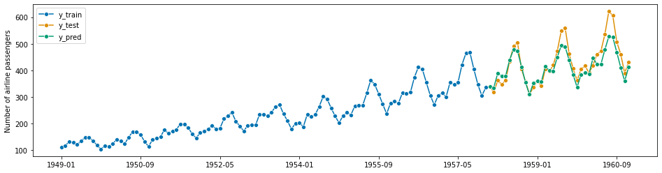
As with scikit-learn models, we can inspect and access parameters of any component via get_params and set_params:
[114]:
forecaster.get_params()
[114]:
{'steps': [('deseasonalize', Deseasonalizer(model='multiplicative', sp=12)),
  ('detrend', Detrender(forecaster=PolynomialTrendForecaster())),
  ('forecast',
   RecursiveTabularRegressionForecaster(estimator=KNeighborsRegressor(),
                                        window_length=15))],
 'deseasonalize': Deseasonalizer(model='multiplicative', sp=12),
 'detrend': Detrender(forecaster=PolynomialTrendForecaster()),
 'forecast': RecursiveTabularRegressionForecaster(estimator=KNeighborsRegressor(),
                                      window_length=15),
 'deseasonalize__model': 'multiplicative',
 'deseasonalize__sp': 12,
 'detrend__forecaster__degree': 1,
 'detrend__forecaster__regressor': None,
 'detrend__forecaster__with_intercept': True,
 'detrend__forecaster': PolynomialTrendForecaster(),
 'forecast__estimator__algorithm': 'auto',
 'forecast__estimator__leaf_size': 30,
 'forecast__estimator__metric': 'minkowski',
 'forecast__estimator__metric_params': None,
 'forecast__estimator__n_jobs': None,
 'forecast__estimator__n_neighbors': 5,
 'forecast__estimator__p': 2,
 'forecast__estimator__weights': 'uniform',
 'forecast__estimator': KNeighborsRegressor(),
 'forecast__transformers': None,
 'forecast__window_length': 15}
sktime provides parameter tuning strategies as compositors of forecaster scitype, similar to scikit-learn’s GridSearchCV.
The compositor ForecastingGridSearchCV (and other tuners) are constructed with a forecaster to tune, a cross-validation constructor, a scikit-learn parameter grid, and parameters specific to the tuning strategy. Cross-validation constructors follow the scikit-learn interface for re-samplers, and can be slotted in exchangeably.
As an example, we show tuning of the window length in the reduction compositor from Section 3.1, using temporal sliding window tuning:
[115]:
from sklearn.neighbors import KNeighborsRegressor

from sktime.forecasting.compose import make_reduction
from sktime.forecasting.model_selection import ForecastingGridSearchCV
from sktime.split import SlidingWindowSplitter
[116]:
regressor = KNeighborsRegressor()
forecaster = make_reduction(regressor, window_length=15, strategy="recursive")
param_grid = {"window_length": [7, 12, 15]}

# We fit the forecaster on an initial window which is 80% of the historical data
# then use temporal sliding window cross-validation to find the optimal hyper-parameters
cv = SlidingWindowSplitter(initial_window=int(len(y_train) * 0.8), window_length=20)
gscv = ForecastingGridSearchCV(
    forecaster, strategy="refit", cv=cv, param_grid=param_grid
)
As with other composites, the resulting forecaster provides the unified interface of sktime forecasters - window splitting, tuning, etc requires no manual effort and is done behind the unified interface:
[117]:
gscv.fit(y_train)
y_pred = gscv.predict(fh)
plot_series(y_train, y_test, y_pred, labels=["y_train", "y_test", "y_pred"])
mean_absolute_percentage_error(y_test, y_pred, symmetric=False)
[117]:
0.16607972017556033

Tuned parameters can be accessed in the best_params_ attribute:
[118]:
gscv.best_params_
[118]:
{'window_length': 7}
An instance of the best forecaster, with hyper-parameters set, can be retrieved by accessing the best_forecaster_ attribute:
[119]:
gscv.best_forecaster_
[119]:
RecursiveTabularRegressionForecaster(estimator=KNeighborsRegressor(),
                                     window_length=7)
As in scikit-learn, parameters of nested components can be tuned by accessing their get_params key - by default this is [estimatorname]__[parametername] if [estimatorname] is the name of the component, and [parametername] the name of a parameter within the estimator [estimatorname].
For example, below we tune the KNeighborsRegressor component’s n_neighbors, in addition to tuning window_length. The tuneable parameters can easily be queried using forecaster.get_params().
[120]:
from sklearn.neighbors import KNeighborsRegressor

from sktime.forecasting.compose import make_reduction
from sktime.forecasting.model_selection import ForecastingGridSearchCV
from sktime.split import SlidingWindowSplitter
[121]:
param_grid = {"window_length": [7, 12, 15], "estimator__n_neighbors": np.arange(1, 10)}

regressor = KNeighborsRegressor()
forecaster = make_reduction(regressor, strategy="recursive")

cv = SlidingWindowSplitter(initial_window=int(len(y_train) * 0.8), window_length=30)
gscv = ForecastingGridSearchCV(forecaster, cv=cv, param_grid=param_grid)
[122]:
gscv.fit(y_train)
y_pred = gscv.predict(fh)
plot_series(y_train, y_test, y_pred, labels=["y_train", "y_test", "y_pred"])
mean_absolute_percentage_error(y_test, y_pred, symmetric=False)
[122]:
0.13988948769413537
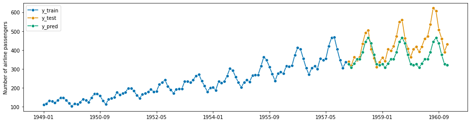
[123]:
gscv.best_params_
[123]:
{'estimator__n_neighbors': 2, 'window_length': 12}
An alternative to the above is tuning the regressor separately, using scikit-learn’s GridSearchCV and a separate parameter grid. As this does not use the “overall” performance metric to tune the inner regressor, performance of the composite forecaster may vary.
[124]:
from sklearn.model_selection import GridSearchCV

# tuning the 'n_estimator' hyperparameter of RandomForestRegressor from scikit-learn
regressor_param_grid = {"n_neighbors": np.arange(1, 10)}
forecaster_param_grid = {"window_length": [7, 12, 15]}

# create a tunnable regressor with GridSearchCV
regressor = GridSearchCV(KNeighborsRegressor(), param_grid=regressor_param_grid)
forecaster = make_reduction(regressor, strategy="recursive")

cv = SlidingWindowSplitter(initial_window=int(len(y_train) * 0.8), window_length=30)
gscv = ForecastingGridSearchCV(forecaster, cv=cv, param_grid=forecaster_param_grid)
[125]:
gscv.fit(y_train)
y_pred = gscv.predict(fh)
plot_series(y_train, y_test, y_pred, labels=["y_train", "y_test", "y_pred"])
mean_absolute_percentage_error(y_test, y_pred, symmetric=False)
[125]:
0.14493362646957736
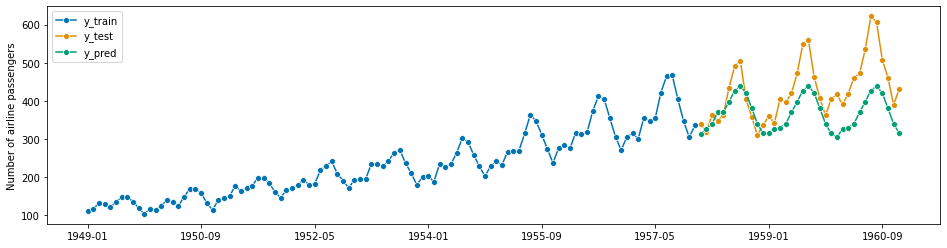
NOTE: a smart implementation of this would use caching to save partial results from the inner tuning and reduce runtime substantially - currently sktime does not support this. Consider helping to improve sktime.
All tuning algorithms in sktime allow the user to set a score; for forecasting the default is mean absolute percentage error. The score can be set using the score argument, to any scorer function or class, as in Section 1.3.
Re-sampling tuners retain performances on individual forecast re-sample folds, which can be retrieved from the cv_results_ argument after the forecaster has been fit via a call to fit.
In the above example, using the mean squared error instead of the mean absolute percentage error for tuning would be done by defining the forecaster as follows:
[126]:
from sktime.performance_metrics.forecasting import MeanSquaredError
[127]:
mse = MeanSquaredError()

param_grid = {"window_length": [7, 12, 15]}

regressor = KNeighborsRegressor()
cv = SlidingWindowSplitter(initial_window=int(len(y_train) * 0.8), window_length=30)

gscv = ForecastingGridSearchCV(forecaster, cv=cv, param_grid=param_grid, scoring=mse)
The performances on individual folds can be accessed as follows, after fitting:
[128]:
gscv.fit(y_train)
gscv.cv_results_
[128]:
| mean_test_MeanSquaredError | mean_fit_time | mean_pred_time | params | rank_test_MeanSquaredError | |
|---|---|---|---|---|---|
| 0 | 2600.750255 | 0.051403 | 0.002837 | {'window_length': 7} | 3.0 |
| 1 | 1134.999053 | 0.051353 | 0.002975 | {'window_length': 12} | 1.0 |
| 2 | 1285.133614 | 0.050748 | 0.003272 | {'window_length': 15} | 2.0 |
sktime provides a number of compositors for ensembling and automated model selection. In contrast to tuning, which uses data-driven strategies to find optimal hyper-parameters for a fixed forecaster, the strategies in this section combine or select on the level of estimators, using a collection of forecasters to combine or select from.
The strategies discussed in this section are: * autoML aka automated model selection * simple ensembling * prediction weighted ensembles with weight updates, and hedging strategies
The most flexible way to perform model selection over forecasters is by using the MultiplexForecaster, which exposes the choice of a forecaster from a list as a hyper-parameter that is tunable by generic hyper-parameter tuning strategies such as in Section 3.3.
In isolation, MultiplexForecaster is constructed with a named list forecasters, of forecasters. It has a single hyper-parameter, selected_forecaster, which can be set to the name of any forecaster in forecasters, and behaves exactly like the forecaster keyed in forecasters by selected_forecaster.
[129]:
from sktime.forecasting.compose import MultiplexForecaster
from sktime.forecasting.exp_smoothing import ExponentialSmoothing
from sktime.forecasting.naive import NaiveForecaster
[130]:
forecaster = MultiplexForecaster(
    forecasters=[
        ("naive", NaiveForecaster(strategy="last")),
        ("ets", ExponentialSmoothing(trend="add", sp=12)),
    ],
)
[131]:
forecaster.set_params(**{"selected_forecaster": "naive"})
# now forecaster behaves like NaiveForecaster(strategy="last")
[131]:
MultiplexForecaster(forecasters=[('naive', NaiveForecaster()),
                                 ('ets',
                                  ExponentialSmoothing(sp=12, trend='add'))],
                    selected_forecaster='naive')
[132]:
forecaster.set_params(**{"selected_forecaster": "ets"})
# now forecaster behaves like ExponentialSmoothing(trend="add", sp=12))
[132]:
MultiplexForecaster(forecasters=[('naive', NaiveForecaster()),
                                 ('ets',
                                  ExponentialSmoothing(sp=12, trend='add'))],
                    selected_forecaster='ets')
The MultiplexForecaster is not too useful in isolation, but allows for flexible autoML when combined with a tuning wrapper. The below defines a forecaster that selects one of NaiveForecaster and ExponentialSmoothing by sliding window tuning as in Section 3.3.
Combined with rolling use of the forecaster via the update functionality (see Section 1.4), the tuned multiplexer can switch back and forth between NaiveForecaster and ExponentialSmoothing, depending on performance, as time progresses.
[133]:
from sktime.forecasting.model_selection import ForecastingGridSearchCV
from sktime.split import SlidingWindowSplitter
[134]:
forecaster = MultiplexForecaster(
    forecasters=[
        ("naive", NaiveForecaster(strategy="last")),
        ("ets", ExponentialSmoothing(trend="add", sp=12)),
    ]
)
cv = SlidingWindowSplitter(initial_window=int(len(y_train) * 0.5), window_length=30)
forecaster_param_grid = {"selected_forecaster": ["ets", "naive"]}
gscv = ForecastingGridSearchCV(forecaster, cv=cv, param_grid=forecaster_param_grid)
[135]:
gscv.fit(y_train)
y_pred = gscv.predict(fh)
plot_series(y_train, y_test, y_pred, labels=["y_train", "y_test", "y_pred"])
mean_absolute_percentage_error(y_test, y_pred, symmetric=False)
[135]:
0.19886711926999853
As with any tuned forecaster, best parameters and an instance of the tuned forecaster can be retrieved using best_params_ and best_forecaster_:
[136]:
gscv.best_params_
[136]:
{'selected_forecaster': 'naive'}
[137]:
gscv.best_forecaster_
[137]:
MultiplexForecaster(forecasters=[('naive', NaiveForecaster()),
                                 ('ets',
                                  ExponentialSmoothing(sp=12, trend='add'))],
                    selected_forecaster='naive')
sktime also provides capabilities for automated selection of pipeline components inside a pipeline, i.e., pipeline structure. This is achieved with the OptionalPassthrough transformer.
The OptionalPassthrough transformer allows to tune whether a transformer inside a pipeline is applied to the data or not. For example, if we want to tune whether sklearn.StandardScaler is bringing an advantage to the forecast or not, we wrap it in OptionalPassthrough. Internally, OptionalPassthrough has a hyperparameter passthrough: bool that is tuneable; when False the composite behaves like the wrapped transformer, when True, it ignores the transformer within.
To make effective use of OptionalPasstrhough, define a suitable parameter set using the __ (double underscore) notation familiar from scikit-learn. This allows to access and tune attributes of nested objects like TabularToSeriesAdaptor(StandardScaler()). We can use __ multiple times if we have more than two levels of nesting.
In the following example, we take a deseasonalize/scale pipeline and tune over the four possible combinations of deseasonalizer and scaler being included in the pipeline yes/no (2 times 2 = 4); as well as over the forecaster’s and the scaler’s parameters.
Note: this could be arbitrarily combined with MultiplexForecaster, as in Section 3.4.1, to select over pipeline architecture as well as over pipeline structure.
Note: scikit-learn and sktime do not support conditional parameter sets at current (unlike, e.g., the mlr3 package). This means that the grid search will optimize over the scaler’s parameters even when it is skipped. Designing/implementing this capability would be an interesting area for contributions or research.
[138]:
from sklearn.preprocessing import StandardScaler

from sktime.datasets import load_airline
from sktime.forecasting.compose import TransformedTargetForecaster
from sktime.forecasting.model_selection import ForecastingGridSearchCV
from sktime.forecasting.naive import NaiveForecaster
from sktime.split import SlidingWindowSplitter
from sktime.transformations.compose import OptionalPassthrough
from sktime.transformations.series.adapt import TabularToSeriesAdaptor
from sktime.transformations.series.detrend import Deseasonalizer
[139]:
# create pipeline
pipe = TransformedTargetForecaster(
    steps=[
        ("deseasonalizer", OptionalPassthrough(Deseasonalizer())),
        ("scaler", OptionalPassthrough(TabularToSeriesAdaptor(StandardScaler()))),
        ("forecaster", NaiveForecaster()),
    ]
)

# putting it all together in a grid search
cv = SlidingWindowSplitter(
    initial_window=60, window_length=24, start_with_window=True, step_length=24
)
param_grid = {
    "deseasonalizer__passthrough": [True, False],
    "scaler__transformer__transformer__with_mean": [True, False],
    "scaler__passthrough": [True, False],
    "forecaster__strategy": ["drift", "mean", "last"],
}
gscv = ForecastingGridSearchCV(forecaster=pipe, param_grid=param_grid, cv=cv)
[140]:
gscv.fit(y_train)
y_pred = gscv.predict(fh)
plot_series(y_train, y_test, y_pred, labels=["y_train", "y_test", "y_pred"])
mean_absolute_percentage_error(y_test, y_pred, symmetric=False)
[140]:
0.1299046419013891
TODO - contributions in this section are appreciated
[141]:
from sktime.forecasting.compose import EnsembleForecaster
[142]:
ses = ExponentialSmoothing(sp=12)
holt = ExponentialSmoothing(trend="add", damped_trend=False, sp=12)
damped = ExponentialSmoothing(trend="add", damped_trend=True, sp=12)

forecaster = EnsembleForecaster(
    [
        ("ses", ses),
        ("holt", holt),
        ("damped", damped),
    ]
)
forecaster.fit(y_train)
y_pred = forecaster.predict(fh)
plot_series(y_train, y_test, y_pred, labels=["y_train", "y_test", "y_pred"])
mean_absolute_percentage_error(y_test, y_pred, symmetric=False)
[142]:
0.16617968035655875
For model evaluation, we sometimes want to evaluate multiple forecasts, using temporal cross-validation with a sliding window over the test data. For this purpose, we can leverage the forecasters from the online_forecasting module which use a composite forecaster, PredictionWeightedEnsemble, to keep track of the loss accumulated by each forecaster and create a prediction weighted by the predictions of the most “accurate” forecasters.
Note that the forecasting task is changed: we make 35 predictions since we need the first prediction to help update the weights, we do not predict 36 steps ahead.
[143]:
from sktime.forecasting.all import mean_squared_error
from sktime.forecasting.online_learning import (
    NormalHedgeEnsemble,
    OnlineEnsembleForecaster,
)
First we need to initialize a PredictionWeightedEnsembler that will keep track of the loss accumulated by each forecaster and define which loss function we would like to use.
[144]:
hedge_expert = NormalHedgeEnsemble(n_estimators=3, loss_func=mean_squared_error)
We can then create the forecaster by defining the individual forecasters and specifying the PredictionWeightedEnsembler we are using. Then by fitting our forecasters and performing updates and prediction with the update_predict function, we get:
[145]:
forecaster = OnlineEnsembleForecaster(
    [
        ("ses", ses),
        ("holt", holt),
        ("damped", damped),
    ],
    ensemble_algorithm=hedge_expert,
)

forecaster.fit(y=y_train, fh=fh)
y_pred = forecaster.update_predict_single(y_test)
plot_series(y_train, y_test, y_pred, labels=["y_train", "y_test", "y_pred"])
mean_absolute_percentage_error(y_test, y_pred, symmetric=False)
[145]:
0.0978975689038194

4. Extension guide - implementing your own forecaster#
sktime is meant to be easily extensible, for direct contribution to sktime as well as for local/private extension with custom methods.
To get started:
Follow the “implementing estimator” developer guide
Use the simple forecasting extension template for forecasters without stream, probabilistic, or hierarchical functionality
Use the advanced forecasting extension template for forecasters with stream, probabilistic or hierarchical functionality
For probabilistic and hierarchical forecasters, it is recommended to familiarize yourself with the interfaces via the tutorials
Read through the forecasting extension template - this is a
pythonfile withtodoblocks that mark the places in which changes need to be added.Optionally, if you are planning any major surgeries to the interface: look at the base class architecture - note that “ordinary” extension (e.g., new algorithm) should be easily doable without this.
Copy the forecasting extension template to a local folder in your own repository (local/private extension), or to a suitable location in your clone of the
sktimeor affiliated repository (if contributed extension), insidesktime.forecasting; rename the file and update the file docstring appropriately.Address the “todo” parts. Usually, this means: changing the name of the class, setting the tag values, specifying hyper-parameters, filling in
__init__,_fit,_predict, and optional methods such as_update(for details see the extension template). You can add private methods as long as they do not override the default public interface. For more details, see the extension template.To test your estimator manually: import your estimator and run it in the workflows in Section 1; then use it in the compositors in Section 3.
To test your estimator automatically: call
sktime.utils.estimator_checks.check_estimatoron your estimator. You can call this on a class or object instance. Ensure you have specified test parameters in theget_test_paramsmethod, according to the extension template.
In case of direct contribution to sktime or one of its affiliated packages, additionally: * Add yourself as an author and/or a maintainer for the new estimator file(s), via "authors" and "maintainers" tag. * Create a pull request that contains only the new estimators (and their inheritance tree, if it’s not just one class), as well as the automated tests as described above. * In the pull request, describe the estimator and optimally provide a publication or other technical
reference for the strategy it implements. * Before making the pull request, ensure that you have all necessary permissions to contribute the code to a permissive license (BSD-3) open source project.
5. Summary#
sktimecomes with several forecasting algorithms (or forecasters), all of which share a common interface. The interface is fully interoperable with thescikit-learninterface, and provides dedicated interface points for forecasting in batch and rolling mode.sktimecomes with rich composition functionality that allows to build complex pipelines easily, and connect easily with other parts of the open source ecosystem, such asscikit-learnand individual algorithm libraries.sktimeis easy to extend, and comes with user friendly tools to facilitate implementing and testing your own forecasters and composition principles.
Useful resources#
For more details, take a look at our paper on forecasting with sktime in which we discuss the forecasting API in more detail and use it to replicate and extend the M4 study.
For a good introduction to forecasting, see Hyndman, Rob J., and George Athanasopoulos. Forecasting: principles and practice. OTexts, 2018.
For comparative benchmarking studies/forecasting competitions, see the M4 competition and the M5 competition.
sktime: sktime/sktime
Generated using nbsphinx. The Jupyter notebook can be found here.